.
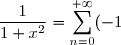
Étant donné une suite de nombres complexes, on lui associe la série de fonctions où : est dite la série entière associée à dont elle est appelée la suite des coefficients.
est dite série entière de la variable réelle si , et de la variable complexe si .
Une série entière de coefficients se note généralement : ou .
II. Convergence d'une série entière
1. Rayon de convergence
Lemme d'Abel :
Soit une série entière et tq est bornée.
Alors, pour tout on a : entraîne converge absolument.
Théorème - Définition :
Soit une série entière. Alors il existe un unique nombre noté avec tq :
s'appelle le rayon de convergence de .
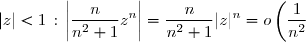
Exemple : :
Pour ; converge absolument.
Pour ; diverge.
Donc
Proposition :
Soit une série entière de rayon de convergence . Alors :
.
.
.
.
.
Notation et vocabulaire : Soit une série entière de rayon de convergence . Alors est appelé le disque de convergence de .
En particulier, si , ; on l'appelle l'intervalle de convergence.
Remarques : 1) Si est la somme de la série entière , alors : .
2) Si :
converge converge.
Ou :
convergence absolument converge absolument.
Alors :
Proposition :
Soit et deux séries entières de rayon de convergence respectivement.
Si , alors : .
Proposition :
Soit et deux séries entières de rayon de convergence respectivement.
S'il existe tq : , alors : .
Proposition :
Soit une fonction rationnelle n'ayant pas de pôles entiers. Alors le rayon de convergence de est égal à 1.
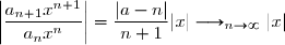
Remarque : L'utilisation de la règle de D'Alembert est pratique surtout pour les séries entières dites lacunaires :
C'est-à-dire les séries de la forme tq une extractrice et : avec
Exemple : avec :
Pour , on pose : .
.
Si (ie ) : donc converge absolument.
Si (ie ) : alors diverge.
On déduit que
Proposition :
Soit une série entière, soit (resp. resp. ) le rayon de convergence de (resp. et ). Alors .
De plus : .
Exemple : avec : :
, donc .
, donc .
On en déduit que .
Proposition :
Soit une série entière de rayon de convergence , soit une fonction rationnelle n'ayant pas de pôles dans .
Alors le rayon de convergence de est égal à .
2. Convergence ponctuelle
Théorème :
Soit une série entière de rayon de convergence .
Alors converge normalement sur tout compact inclus dans
Remarque : Il se peut qu'une série entière de rayon de convergence positif ne converge pas normalement sur le disque .
Corollaire :
La somme d'une série entière de rayon de convergence positif est continue sur le disque .
III. Opérations sur les séries entières
Soit , deux séries entières de rayons de convergence et respectivement.
Soit .
On pose : , et .
On note et les rayons de convergence respectivement des séries entières : , et .
i) .
.
ii) .
iii) .
.
IV. Propriétés de la somme d'une série entière de la variable réelle
Ici, est une série entière de la variable réelle dont le rayon de convergence est supposé positif et dont la somme est noté .
est définie sur au moins , on rappelle que est continue sur cet intervalle.
Théorème :
La série entière est de rayon de convergence
De plus, on a : .
Remarque : Soit .
.
Autrement dit : .
On dit qu'une série entière s'intègre terme à terme entre deux points quelconques de son intervalle de convergence .
Théorème :
Pour tout , la série entière a pour rayon de convergence .
est de classe sur et on a : : .
Exemple : Soit .
On a : ; est donc définie et continue sur .
et existent, donc : .
.
converge, donc est somme uniforme sur d'une série de fonctions continue sur , alors est continue sur .
est de classe sur :
et .
(car ).
Donc : .
et puisque ,
.
Donc : .
Remarque : On avait obtenu : .
Donc : , on en déduit : .
Essayons de démontrer ce résultat directement en étudiant la somme partielle de la série :
Soit On conclut que la méthode des séries entières est plus performante que la méthode directe.
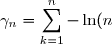
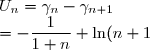
Rappel : La constante d'Euler On pose : Etudions la convergence de la suite en introduisant la série téléscopique tq :
Donc : .
La suite étant réelle, à partir d'un certain rang ( est à terme positif à partir du rang ) .
Donc : converge, alors : converge.
On en déduit que : converge.
Définition :
La limite de la suite est appelée la constante d'Euler, on la note .
Remarque : On a :, d'où :
V. Développement en série entière (DSE)
1. Généralités
est un intervalle de tq .
Définition :
Soit et tq :.
On dit que est développable en série entière (DSE) sur ssi il existe une série entière de rayon de convergence tq : : .
De manière plus générale si et si on dit que f est développable en série entière au voisinage de s'il existe tel que et une série entière de rayon de convergence tels que
Définition :
Soit , on dit que DSE au voisinage de ssi il existe tq : On note : .
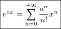
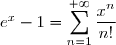
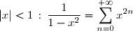
Exemples : La fonction est DSE sur avec : .
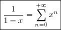
La fonction est DSE sur avec : .
Soit , :
est définie sur .
Sur cet intervalle, est DSE.
En effet, Or : D'où : , donc : .
Soit polynômiale de degré :
Alors : avec et .
En posant .
converge pour tout de somme .
Toute fonction polynômiale est DSE sur et elle est son propre développement.
Théorème :
Soit DSE sur avec . Alors :
est de classe sur .
.
Exemple : Soit ; on a : D'où : .
Si C'est-à-dire : .
Et cela reste vrai pour ; donc .
On conclut que est DSE sur donc sur .
Corollaire :
Soit et tq : .
Si est DSE sur avec . Alors est unique.
Exemple : Soit Méthode 1 : Pour et .
D'où, pour avec : D'où : , pour Donc la méthode 1) nous fournit : pour .
Méthode 2 : On a : et pour : .
Or, .
On obtient : .
Donc la méthode 2) nous fournit : .
Méthode 3 : Décomposons en fractions rationnelles : On obtient par calcul : .
La méthode nous fournit : Par unicité du DSE sur , on a :
Définiton :
Soit de classe .
La série entière est appelée la série de Taylor de .
2. Techniques de calcul de DSE au voisinage de 0
Il existe plusieurs méthodes de calcul d'un DSE d'une fonction, nous citerons ici les plus utilisées, mais cela ne veut pas dire qu'elles sont les seules, on peut très bien avoir affaire à d'autres méthodes.
Notations et vocabulaire : Si (avec ) est un DSE sur alors le rayon de convergence de la série entière est appelé le rayon de convergence du DSE de .
Le plus grand intervalle ouvert sur lequel ce développement est valable s'appelle le domaine de validité du DSE de , on le note .
Remarque : en général. (Avec est le domaine de validité d'un DSE de ).
Contre exemple : on a : et .
Technique 1 : Utilisation des opérations sur les séries entières
Supposons : , et , En posant , on a :
: ; pour .
; pour .
Donc toute combinaison linéaire (resp. produit) de deux fonctions DSE(0) est une fonction DSE(0).
Exemples : :
On a : De plus : donc : Alors : Donc : De même : :
On a : :
On a : et Alors : .
On conclut : De même :
Technique 2 : Méthode de la dérivation et intégration
Soit dérivable tq admet un DSE sur donné par : .
Alors : .
D'où, .
Exemples : est dérivable et .
Or pour tout tq : .
D'où : avec .
C'est-à-dire : .
est dérivable sur et .
On a : avec .
D'où : Donc : .
Technique 3 : Utilisation d'une équation differentielle linéaire
On considère l'équation différentielle linéaire d'ordre :
où : .
Etant donné et , on admet qu'il existe une unique solution de sur tq :
Soit de classe .
Si on détermine toutes les solutions de , DSE(0) et si l'une d'elle, , vérifie :
Alors , d'où est DSE(0).
Dans la pratique, on se contentera du cas où les fonctions sont rationnelles.
Exemple : est dérivable et .
est donc solution sur de l'équation différentielle .
Soit , soit de classe et DSE sur .
Posons : avec .
.
On a :
est solution de sur .
Par unicité du DSE sur de la fonction nulle.
est solution de sur
Remarque : Formellement : . On pouvait donc prendre .
est solution de sur Or, .
On a donc trouvé le DSE de sur et qui est :
Publié par Panter
le
ceci n'est qu'un extrait
Pour visualiser la totalité des cours vous devez vous inscrire / connecter (GRATUIT) Inscription Gratuitese connecter
Merci à Panter pour avoir contribué à l'élaboration de cette fiche
Désolé, votre version d'Internet Explorer est plus que périmée ! Merci de le mettre à jour ou de télécharger Firefox ou Google Chrome pour utiliser le site. Votre ordinateur vous remerciera !
 .
.
_{n \in \mathbb{N}}) de nombres complexes, on lui associe la série de fonctions
de nombres complexes, on lui associe la série de fonctions  où :
où : 
 , et de la variable complexe si
  .
.
) se note généralement :
se note généralement :  ou
ou  .
.
 :
:
) ;
;  converge absolument.
![|z| > 1 \, : \, \left|\displaystyle \frac{n}{n^2+1} z^n \right| = \displaystyle \frac{n}{n^2+1} |z|^n \xrightarrow[n\to+\infty]{} +\infty](https://latex.ilemaths.net/latex-0.tex?|z| > 1 \, : \, \left|\displaystyle \frac{n}{n^2+1} z^n \right| = \displaystyle \frac{n}{n^2+1} |z|^n \xrightarrow[n\to+\infty]{} +\infty) ;
; 
 . Alors
  = \lbrace z \in \mathbb{K} / |z| < R \rbrace) est appelé le disque de convergence de
est appelé le disque de convergence de ![D(0,R) = ]-R , R[](https://latex.ilemaths.net/latex-0.tex?D(0,R) = ]-R , R[) ; on l'appelle l'intervalle de convergence.
; on l'appelle l'intervalle de convergence.
 est la somme de la série entière
  , alors :
  \subset D_f \subset \overline{D(0 , R)}) .
.
 :
:

 converge.
 converge absolument.
 = R_{cv} \left( \displaystyle \sum_{n \geq 0} b_n z^n \right))
}) tq
tq  une extractrice et :
 } = \displaystyle \sum_{n \geq 0} a_n z^n) avec
avec } = b \\ a_k = 0 \text{ si } k \not \in \psi(\mathbb{N})} \end{array} \right .)
 avec
avec  :
:
 , on pose :
  = \displaystyle \frac{na^n}{2^n} z^{3n}) .
.
![\forall n \geq 1 \, : \, \left| \displaystyle \frac{b_{n+1}(z)}{b_n(z)} \right| = \left| \displaystyle \frac{n+1}{n} \frac{a}{2} z^3 \right| = \displaystyle \frac{n+1}{n} \frac{|a|}{2} |z|^3 \xrightarrow[n\to+\infty]{} \displaystyle \frac{|a|}{2} |z|^3](https://latex.ilemaths.net/latex-0.tex?\forall n \geq 1 \, : \, \left| \displaystyle \frac{b_{n+1}(z)}{b_n(z)} \right| = \left| \displaystyle \frac{n+1}{n} \frac{a}{2} z^3 \right| = \displaystyle \frac{n+1}{n} \frac{|a|}{2} |z|^3 \xrightarrow[n\to+\infty]{} \displaystyle \frac{|a|}{2} |z|^3) .
.
 (ie
(ie ^{\frac{1}{3}}) ) : donc
) : donc  converge absolument.
 (ie
(ie ^{\frac{1}{3}}) ) : alors
) : alors  diverge.
^{\frac{1}{3}})
 avec :
 ^n}) :
:
 , donc
  .
.
 , donc
  .
.
 .
.
) .
.
 et
et  respectivement.
 .
.
 ,
,  et
et  .
.
 et
et  les rayons de convergence respectivement des séries entières :
  ,
,  et
et  .
.
) .
.
 \, \Longrightarrow \, \displaystyle \sum_{n=0}^{+\infty}(a_n + b_n)z^n = \displaystyle \sum_{n=0}^{+\infty} a_n z^n + \displaystyle \sum_{n=0}^{+\infty} b_n z^n) .
.

 .
.
) .
.
 \, \Longrightarrow \, \displaystyle \sum_{n=0}^{+\infty} \left(\displaystyle \sum_{k=0}^n a_k b_{n-k} \right)z^n = \left(\displaystyle \sum_{n=0}^{+\infty} a_n z^n \right) \left(\displaystyle \sum_{n=0}^{+\infty} b_n z^n \right)) .
.
 est une série entière de la variable réelle dont le rayon de convergence
 ![]-R , R[](https://latex.ilemaths.net/latex-0.tex?]-R , R[) , on rappelle que
, on rappelle que ![\forall x \in ]-R,R[ \, : \, \displaystyle \sum_{n=0}^{+\infty} a_n \displaystyle \frac{x^{n+1}}{n+1} = \displaystyle \int_0^{x} f(t) \text{d}t](https://latex.ilemaths.net/latex-0.tex?\forall x \in ]-R,R[ \, : \, \displaystyle \sum_{n=0}^{+\infty} a_n \displaystyle \frac{x^{n+1}}{n+1} = \displaystyle \int_0^{x} f(t) \text{d}t) .
.
![p , q \in ]-R , R[ \, : \, \displaystyle \int_{p}^q f(t) \text{d}t = \displaystyle \int_{0}^q f(t) \text{d}t - \displaystyle \int_{0}^p f(t) \text{d}t](https://latex.ilemaths.net/latex-0.tex?p , q \in ]-R , R[ \, : \, \displaystyle \int_{p}^q f(t) \text{d}t = \displaystyle \int_{0}^q f(t) \text{d}t - \displaystyle \int_{0}^p f(t) \text{d}t) .
.
 \text{d}t = \displaystyle \sum_{n=0}^{+\infty} a_n \displaystyle \frac{q^{n+1}}{n+1} - \displaystyle \sum_{n=0}^{+\infty} a_n \displaystyle \frac{p^{n+1}}{n+1} = \displaystyle \sum_{n=0}^{+\infty} a_n \displaystyle \frac{q^{n+1}-p^{n+1}}{n+1} = \displaystyle \sum_{n=0}^{+\infty} \displaystyle \int_{p}^q a_n t^n \text{d}t) .
.
 \text{d}t = \displaystyle \sum_{n=0}^{+\infty} \left(\displaystyle \int_p^q a_n t^n \text{d}t\right)) .
.
 = \displaystyle \sum_{n=2}^{+\infty} \displaystyle \frac{x^n}{n(n-1)}) .
.
 ;
; ![]-1 , 1[](https://latex.ilemaths.net/latex-0.tex?]-1 , 1[) .
.
) et
et ) existent, donc :
existent, donc : ![D_f = [-1 , 1]](https://latex.ilemaths.net/latex-0.tex?D_f = [-1 , 1]) .
.
![\forall n \geq 2 \, , \, \forall x \in [-1,1] \, : \, \left| \displaystyle \frac{x^n}{n(n-1)} \right| \leq \displaystyle \frac{1}{n(n-1)} = \alpha_n](https://latex.ilemaths.net/latex-0.tex?\forall n \geq 2 \, , \, \forall x \in [-1,1] \, : \, \left| \displaystyle \frac{x^n}{n(n-1)} \right| \leq \displaystyle \frac{1}{n(n-1)} = \alpha_n) .
.
 converge, donc
 ![[-1 , 1]](https://latex.ilemaths.net/latex-0.tex?[-1 , 1]) d'une série de fonctions continue sur
d'une série de fonctions continue sur ![[-1,1]](https://latex.ilemaths.net/latex-0.tex?[-1,1]) .
.
 sur
sur ![]-1,1[](https://latex.ilemaths.net/latex-0.tex?]-1,1[) :
:
 = \displaystyle \sum_{n=2}^\infty \frac{x^{n-1}}{n-1}) et
et  = \displaystyle \sum_{n=2}^{+\infty} x^{n-2} = \displaystyle \sum_{n=0}^{+\infty} x^n = \displaystyle \frac{1}{1-x}) .
.
 = \displaystyle \int_{0}^x f''(t) \text{d}t) (car
(car  = 0) ).
).
 = \displaystyle \int_{0}^x f''(t) \text{d}t = \displaystyle \int_{0}^x \displaystyle \frac{\text{d}t}{1-t} = -\ln(1-x)) .
.
 = 0) ,
,
![f(x) = \displaystyle \int_{0}^x f'(t) \text{d}t = (1 - x) \ln(1 - x) + x \hspace{20pt} \forall x \in ]-1 , 1[](https://latex.ilemaths.net/latex-0.tex?f(x) = \displaystyle \int_{0}^x f'(t) \text{d}t = (1 - x) \ln(1 - x) + x \hspace{20pt} \forall x \in ]-1 , 1[) .
.
![\boxed{f(x) = \displaystyle \sum_{n=2}^{+\infty} \displaystyle \frac{x^n}{n(n-1)} = (1 - x)\ln(1 - x) + x \hspace{20pt} \forall x \in ]-1 , 1[}](https://latex.ilemaths.net/latex-0.tex?\boxed{f(x) = \displaystyle \sum_{n=2}^{+\infty} \displaystyle \frac{x^n}{n(n-1)} = (1 - x)\ln(1 - x) + x \hspace{20pt} \forall x \in ]-1 , 1[}) .
.
![\forall x \in ]-1 , 1[ \, : \, \displaystyle \sum_{n=2}^{+\infty} \displaystyle \frac{x^n}{n(n-1)} = (1-x)\ln(1-x) + x](https://latex.ilemaths.net/latex-0.tex?\forall x \in ]-1 , 1[ \, : \, \displaystyle \sum_{n=2}^{+\infty} \displaystyle \frac{x^n}{n(n-1)} = (1-x)\ln(1-x) + x) .
.
 = \displaystyle \lim_{n\to-1^+} f(x) = 2\ln 2 -1) , on en déduit :
, on en déduit : ^n}{n(n-1)} = 2\ln2-1) .
.

^n}{n(n-1)} \\ = \displaystyle \sum_{k=1}^{N} \displaystyle \frac{1}{2k(2k-1)} - \displaystyle \sum_{k=1}^{N} \frac{1}{2k(2k+1)} \\ = \displaystyle \sum_{k=1}^{N} \left(\displaystyle \frac{1}{2k-1} - \displaystyle \frac{1}{2k}\right) - \displaystyle \sum_{k=1}^{N} \left(\displaystyle \frac{1}{2k} - \displaystyle \frac{1}{2k+1}\right)\\ = \displaystyle \sum_{k=1}^{N} \displaystyle \frac{1}{2k-1} + \displaystyle \sum_{k=1}^{N} \displaystyle \frac{1}{2k+1} - \displaystyle \sum_{k=1}^{N} \displaystyle \frac{1}{k})
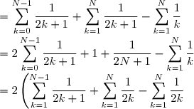 + 1 + \displaystyle \frac{1}{2N+1} - \displaystyle \sum_{k=1}^{N} \displaystyle \frac{1}{k})
![= 2 \left(\displaystyle \sum_{k=1}^{2N} \displaystyle \frac{1}{k}\right) - 2 \displaystyle \sum_{k=1}^{N} \displaystyle \frac{1}{k} - 2 + 1 + \displaystyle \frac{1}{2N + 1} \\ = 2 \left(\gamma_{2N} +\ln (2N)\right) - 2 \left(\gamma_N + \ln N\right) - 1 + \displaystyle \frac{1}{2N+1} \\ = 2 \gamma_{2N} - 2\gamma_{N} + 2\ln 2 - 1 + \displaystyle \frac{1}{2N+1} \xrightarrow[N \to +\infty]{} 2\ln2-1](https://latex.ilemaths.net/latex-0.tex?= 2 \left(\displaystyle \sum_{k=1}^{2N} \displaystyle \frac{1}{k}\right) - 2 \displaystyle \sum_{k=1}^{N} \displaystyle \frac{1}{k} - 2 + 1 + \displaystyle \frac{1}{2N + 1} \\ = 2 \left(\gamma_{2N} +\ln (2N)\right) - 2 \left(\gamma_N + \ln N\right) - 1 + \displaystyle \frac{1}{2N+1} \\ = 2 \gamma_{2N} - 2\gamma_{N} + 2\ln 2 - 1 + \displaystyle \frac{1}{2N+1} \xrightarrow[N \to +\infty]{} 2\ln2-1)
)
) en introduisant la série téléscopique
en introduisant la série téléscopique  tq :
tq :
-\ln(n) \\ = - \displaystyle \frac{1}{n} \displaystyle \frac{1}{1 + \frac{1}{n}} + \ln \left(1+\frac{1}{n}\right) \\ = - \displaystyle \frac{1}{n} \left(1 - \displaystyle \frac{1}{n} + o \left(\displaystyle \frac{1}{n} \right) \right) + \left(\displaystyle \frac{1}{n} - \displaystyle \frac{1}{2n^2} + o \left(\displaystyle \frac{1}{n^2}\right)\right) \\ = \displaystyle \frac{1}{2n^2} + o \left(\displaystyle \frac{1}{n^2}\right))
 .
.
 à partir d'un certain rang
  (
( converge, alors :
  converge.
 - \gamma = o(1)) , d'où :
, d'où :  +\gamma + o(1))
 est un intervalle de
  tq
tq  .
.
 .
.
![\begin{array}{rccl} f : & ]-\infty , 1[ & \longrightarrow & \mathbb{R} \\ & x & \mapsto & \displaystyle \frac{1}{1-x} \\ \end{array}](https://latex.ilemaths.net/latex-0.tex?\begin{array}{rccl} f : & ]-\infty , 1[ & \longrightarrow & \mathbb{R} \\ & x & \mapsto & \displaystyle \frac{1}{1-x} \\ \end{array})
 .
.
 ,
,  :
:
![]-|a| , |a|[](https://latex.ilemaths.net/latex-0.tex?]-|a| , |a|[) .
.
 = \displaystyle \frac{1}{a} \left( \displaystyle \frac{1}{1 - \displaystyle \frac{x}{a}} \right))

 = \displaystyle \frac{1}{a} \displaystyle \sum_{n=0}^{+\infty} \left(\frac{x}{a} \right)^n) , donc :
, donc : 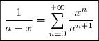 .
.
 polynômiale de degré
  :
:
 = a_0 + a_1x + \cdots + a_px^p) avec
avec  et
et  .
.
 .
.
 de somme
 ) .
.


 .
.
!})
 = \displaystyle \sum_{n=0}^{+\infty} \displaystyle \frac{x^n}{(n+1)^!}) .
.
 ; donc
  = \displaystyle \sum_{n=0}^{+\infty} \displaystyle \frac{x^n}{(n+1)^!}) .
.
 sur
sur ![\begin{array}{rccl} f: & ]-1,1[ & \longrightarrow & \mathbb{R} \\ & x & \mapsto & \displaystyle \frac{1}{(1-x^2)(1+x)} \\ \end{array}](https://latex.ilemaths.net/latex-0.tex?\begin{array}{rccl} f: & ]-1,1[ & \longrightarrow & \mathbb{R} \\ & x & \mapsto & \displaystyle \frac{1}{(1-x^2)(1+x)} \\ \end{array})
 et
et 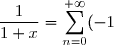^n x^n) .
.
 = \left(\displaystyle \sum_{n=0}^{+\infty} x^{2n}\right) \left(\displaystyle \sum_{n=0}^{+\infty} (-1)^n x^n \right))
 \left(\displaystyle \sum_{n=0}^{+\infty} (-1)^n x^n \right)) avec :
avec : 
 = \displaystyle \sum_{n=0}^{+\infty} \left(\displaystyle \sum_{k=0}^{n} a_k (-1)^{n-k} \right) x^n = \displaystyle \sum_{n=0}^{+\infty} \left(\displaystyle \sum_{k=0}^{E(\frac{n}{2})} a_{2k} (-1)^{n-2k} \right) x^n) , pour
, pour 
 = \displaystyle \sum_{n=0}^{+\infty} (-1)^n \left(E \left(\displaystyle \frac{n}{2} \right) + 1 \right) x^n}) pour
pour  = \displaystyle \frac{1}{(1-x)(1+x)^2}) et pour
et pour  .
.
^2} = \left(\frac{-1}{x+1}\right)' = -\left(\displaystyle \sum_{n=0}^{+\infty} (-1)^n x^n \right)' = -\displaystyle \sum_{n=1}^{+\infty} (-1)^{n} n x^{n-1} =\displaystyle \sum_{n=1}^{+\infty} (-1)^{n+1} n x^{n-1}) .
.
^2} = \displaystyle \sum_{n=0}^{+\infty} (-1)^{n} (n+1) x^{n}) .
.
 = \left( \displaystyle \sum_{n=0}^{+\infty}x^n \right) \left(\displaystyle \sum_{n=0}^{+\infty} (-1)^{n} (n+1) x^{n} \right))
 = \displaystyle \sum_{n=0}^{+\infty} \left(\displaystyle \sum_{n=0}^{n} (-1)^{k} (k+1) \right) x^{n}}) .
.
 = \displaystyle \frac{a}{1-x} + \displaystyle \frac{b}{1+x} + \displaystyle \frac{c}{(1+x)^2})
 = 1 = a + b + c \right))
 = \displaystyle \frac{1}{4(1-x)} + \displaystyle \frac{1}{4(1+x)} + \displaystyle \frac{1}{2(1+x)^2} \\ = \frac{1}{4} \displaystyle \sum_{n=0}^{+\infty} x^n + \displaystyle \frac{1}{4} \displaystyle \sum_{n=0}^{+\infty} (-1)^n x^n + \displaystyle \frac{1}{2} \displaystyle \sum_{n=0}^{+\infty} (-1)^n (n+1)x^n \\ = \displaystyle \sum_{n=0}^{+\infty} \displaystyle \frac{1+(-1)^n+2(-1)^n(n+1)}{4} x^n = \displaystyle \sum_{n=0}^{+\infty} \displaystyle \frac{1+(-1)^n(2n+3)}{4} x^n) .
.
 = \displaystyle \sum_{n=0}^{+\infty} \displaystyle \frac{1+(-1)^n(2n+3)}{4} x^n})
^n \left(E \left(\displaystyle \frac{n}{2} \right) + 1\right) = \displaystyle \sum_{k=0}^n (-1)^k (k+1) = \displaystyle \frac{1+(-1)^n(2n+3)}{4}})
 = \displaystyle \sum_{n=0}^{+\infty} a_n x^n) (avec
(avec  ) est un DSE sur
 ![]-r , r[](https://latex.ilemaths.net/latex-0.tex?]-r , r[) alors le rayon de convergence de la série entière
alors le rayon de convergence de la série entière  .
.
 en général. (Avec
  on a :
 ![D_v = ]-1 , 1[](https://latex.ilemaths.net/latex-0.tex?D_v = ]-1 , 1[) et
et  .
.
 et
et  = \displaystyle \sum_{n=0}^{+\infty} b_n x^n) ,
, 
) , on a :
, on a :
 :
:  + \eta g(x) = \displaystyle \sum_{n=0}^{+\infty} \left(\lambda a_n + \eta b_n \right) x^n) ;
;  pour
pour  = \displaystyle \sum_{n=0}^{+\infty} \left(\displaystyle \sum_{k=0}^{n} a_k b_{n-k} \right) x^n) ;
;  \text{ et } x \longrightarrow sh(x)) :
:
 = \frac{e^x+e^{-x}}{2})
^n}{n!} x^n)
^n}{2} \frac{x^n}{n!} \, \, \forall x \in \mathbb{R})
!} \, , \, x \in \mathbb{R}})
!} \, , \, x \in \mathbb{R}})
 :
:
 = \displaystyle \frac{e^{ix}+e^{-ix}}{2}) :
:
 et
et ^n x^n}{n!})
 = \displaystyle \sum_{n=0}^{+\infty} \displaystyle \frac{i^n +(-i)^n}{2} \displaystyle \frac{x^n}{n!} = \displaystyle \sum_{n=0}^{+\infty}i^{2n} \displaystyle \frac{x^{2n}}{2n!}) .
.
 = \displaystyle \sum_{n=0}^{+\infty} (-1)^n \displaystyle \frac{x^{2n}}{(2n)!} \, , \, x \in \mathbb{R}})
 = \displaystyle \sum_{n=0}^{+\infty} (-1)^n \displaystyle \frac{x^{2n+1}}{(2n+1)!} \, , \, x \in \mathbb{R}})
 dérivable tq
  admet un DSE sur
 ![]-r , r[ \subset I](https://latex.ilemaths.net/latex-0.tex?]-r , r[ \subset I) donné par :
donné par :  = \displaystyle \sum_{n=0}^{+\infty} a_n x^n) .
.
![\displaystyle \int_{0}^x f'(t)dt = \displaystyle \sum_{n=0}^{+\infty} \displaystyle \frac{a_n}{n+1} x^{n+1} \, , \, \forall x \in ]-r , r[](https://latex.ilemaths.net/latex-0.tex?\displaystyle \int_{0}^x f'(t)dt = \displaystyle \sum_{n=0}^{+\infty} \displaystyle \frac{a_n}{n+1} x^{n+1} \, , \, \forall x \in ]-r , r[) .
.
![\forall x \in ]-r , r[ \, : \, f(x) = f(0) + \displaystyle \sum_{n=0}^{+\infty} \displaystyle \frac{a_n}{n+1}x^{n+1}](https://latex.ilemaths.net/latex-0.tex?\forall x \in ]-r , r[ \, : \, f(x) = f(0) + \displaystyle \sum_{n=0}^{+\infty} \displaystyle \frac{a_n}{n+1}x^{n+1}) .
.
![\begin{array}{rccl} f : & ]-1 , +\infty[ & \longrightarrow & \mathbb{R} \\ & x & \mapsto & \ln(1+x) \\ \end{array}](https://latex.ilemaths.net/latex-0.tex?\begin{array}{rccl} f : & ]-1 , +\infty[ & \longrightarrow & \mathbb{R} \\ & x & \mapsto & \ln(1+x) \\ \end{array})
![f'(x) = \displaystyle \frac{1}{1+x} \, \forall x \in ]-1 , +\infty[](https://latex.ilemaths.net/latex-0.tex?f'(x) = \displaystyle \frac{1}{1+x} \, \forall x \in ]-1 , +\infty[) .
.
^n x^n) pour tout
pour tout  tq :
tq :  = f(0) + \displaystyle \sum_{n=0}^{+\infty} \displaystyle \frac{(-1)^n}{n+1} x^{n+1}) avec
avec  = \displaystyle \sum_{n=1}^{+\infty} \displaystyle \frac{(-1)^{n-1} x^n}{n} \, , \, |x| < 1}) .
.
\\ \end{array})
 = \displaystyle \frac{1}{1+x^2}) .
.
^n x^{2n}) avec
avec  = f(0) + \displaystyle \sum_{n=0}^{+\infty} \displaystyle \frac{(-1)^n}{2n+1} x^{2n+1})
 = \displaystyle \sum_{n=0}^{+\infty} \displaystyle \frac{(-1)^n}{2n+1} x^{2n+1} \, , \, |x| < 1}) .
.
 :
:
 : y^{(n)} + a_{n-1}(x) y^{(n-1)} +\cdots + a_0(x) y = b(x)) où :
où : ) .
.
 et
et  , on admet qu'il existe une unique solution
 ) sur
sur  & = & c_0 \\ \psi '(x_0) & = & c_1\\ \vdots & & \\ \psi^{(n-1)}(x_0) & = & c_{n-1} \\ \end{array} \right \rbrace )
 & = & f(0) \\ \psi '(0) & = & f'(0) \\ \vdots & & \\ \psi^{(n-1)}(0) & = & f^{(n-1)}(0) \\ \end{array} \right \rbrace )
 , d'où
  sont rationnelles.
![\begin{array}{rccl} f : & ]-1 , +\infty[ & \longrightarrow& \mathbb{C} \\ & x & \mapsto & (1+x)^a \\ \end{array} (a \in \mathbb{C} \backslash \mathbb{Z} )](https://latex.ilemaths.net/latex-0.tex? \begin{array}{rccl} f : & ]-1 , +\infty[ & \longrightarrow& \mathbb{C} \\ & x & \mapsto & (1+x)^a \\ \end{array} (a \in \mathbb{C} \backslash \mathbb{Z} ))
 = a(1 + x)^{a - 1}) .
.
f'(x) = a(1 + x)^a = af(x))
![]-1 , +\infty[](https://latex.ilemaths.net/latex-0.tex?]-1 , +\infty[) de l'équation différentielle
de l'équation différentielle  : (1+x)y' - ay = 0 \Longleftrightarrow y' - \displaystyle \frac{a}{x+1} y = 0) .
.
![r \in ]0 , 1]](https://latex.ilemaths.net/latex-0.tex?r \in ]0 , 1]) , soit
, soit ![\psi : ]-r , r[ \longrightarrow \mathbb{C}](https://latex.ilemaths.net/latex-0.tex?\psi : ]-r , r[ \longrightarrow \mathbb{C}) de classe
de classe  = \displaystyle \sum_{n=0}^{+\infty} a_n x^{n}) avec
avec  = \displaystyle \sum_{n=1}^{+\infty} n a_nx^{n-1}) .
.
) sur
sur ![\Longleftrightarrow \, \forall x \in ]-r , r[ \, : \, (1 + x) \displaystyle \sum_{n=1}^{+\infty} n a_n x^{n-1} - a \displaystyle \sum_{n=0}^{+\infty} a_n x^n = 0](https://latex.ilemaths.net/latex-0.tex?\Longleftrightarrow \, \forall x \in ]-r , r[ \, : \, (1 + x) \displaystyle \sum_{n=1}^{+\infty} n a_n x^{n-1} - a \displaystyle \sum_{n=0}^{+\infty} a_n x^n = 0)
![\Longleftrightarrow \, \forall x \in ]-r , r[ \, : \, \displaystyle \sum_{n=1}^{+\infty} na_n x^{n-1} + \displaystyle \sum_{n=1}^{+\infty} n a_n x^n - a \displaystyle \sum_{n=0}^{+\infty} a_n x^n = 0 \\ \Longleftrightarrow \, \forall x \in ]-r , r[ \, : \, \displaystyle \sum_{n=0}^{+\infty} (n+1)a_{n+1} x^n + \displaystyle \sum_{n=1}^{+\infty} n a_n x^n - a\displaystyle \sum_{n=0}^{+\infty} a_n x^n = 0 \\ \Longleftrightarrow \forall x \in ]-r , r[ \, : \, \displaystyle \sum_{n=0}^{+\infty} \left[(n + 1) a_{n+1} - (a - n)a_n \right] x^n = 0](https://latex.ilemaths.net/latex-0.tex?\Longleftrightarrow \, \forall x \in ]-r , r[ \, : \, \displaystyle \sum_{n=1}^{+\infty} na_n x^{n-1} + \displaystyle \sum_{n=1}^{+\infty} n a_n x^n - a \displaystyle \sum_{n=0}^{+\infty} a_n x^n = 0 \\ \Longleftrightarrow \, \forall x \in ]-r , r[ \, : \, \displaystyle \sum_{n=0}^{+\infty} (n+1)a_{n+1} x^n + \displaystyle \sum_{n=1}^{+\infty} n a_n x^n - a\displaystyle \sum_{n=0}^{+\infty} a_n x^n = 0 \\ \Longleftrightarrow \forall x \in ]-r , r[ \, : \, \displaystyle \sum_{n=0}^{+\infty} \left[(n + 1) a_{n+1} - (a - n)a_n \right] x^n = 0) .
.
![]-r , r[ \, \Longleftrightarrow \, \forall n \in \mathbb{N} \, : \, a_{n+1} = \displaystyle \frac{a-n}{n+1} a_n \, \, (*)](https://latex.ilemaths.net/latex-0.tex?]-r , r[ \, \Longleftrightarrow \, \forall n \in \mathbb{N} \, : \, a_{n+1} = \displaystyle \frac{a-n}{n+1} a_n \, \, (*))
 . On pouvait donc prendre
  .
.
 \, \Longleftrightarrow \, \forall n \in \mathbb{N}^* \, : \, a_n = \displaystyle \frac{a(a-1) \cdots (a-n+1)}{n!} a_0 = {{a}\choose {n}} a_0)
![]-r , r[ \, \Longleftrightarrow \, \forall x\in]-r , r[ \, : \, \psi(x) = a_0 \displaystyle \sum_{n=0}^{+\infty} {a\choose n} x^n](https://latex.ilemaths.net/latex-0.tex?]-r , r[ \, \Longleftrightarrow \, \forall x\in]-r , r[ \, : \, \psi(x) = a_0 \displaystyle \sum_{n=0}^{+\infty} {a\choose n} x^n)
 = f(0) \, \Longleftrightarrow \, a_0 = 1) .
.
^a = \displaystyle \sum_{n=0}^{+\infty} {a\choose n} x^n}) Publié par Panter
le
Publié par Panter
le
 une série entière et
  tq
tq _n) est bornée.
est bornée.
 on a :
  entraîne
  une série entière. Alors il existe un unique nombre noté
  tq :
tq :
 \text{ bornée } \rbrace ) .
.
 .
.
 .
.
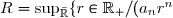
![R = \sup_{\bar{\mathbb{R}}} \lbrace |z| / z \in \mathbb{K} \text{ et } a_nz^n \xrightarrow[n \to +\infty]{} 0 \rbrace](https://latex.ilemaths.net/latex-0.tex?R = \sup_{\bar{\mathbb{R}}} \lbrace |z| / z \in \mathbb{K} \text{ et } a_nz^n \xrightarrow[n \to +\infty]{} 0 \rbrace) .
.
 \text{ converge } \rbrace ) .
.
 respectivement.
 , alors :
  .
.
 tq :
tq :  , alors :
  .
.
z^n) est égal à 1.
est égal à 1.
 resp.
resp.  ) le rayon de convergence de
  et
et  ). Alors
 ) .
.
 .
.
 .
.
 a_n z^n) est égal à
est égal à  .
.
 est de rayon de convergence
  , la série entière
 !} x^{n-k}) a pour rayon de convergence
a pour rayon de convergence ![\forall k \in \mathbb{N} \, , \, \forall x \in ]-R , R[](https://latex.ilemaths.net/latex-0.tex?\forall k \in \mathbb{N} \, , \, \forall x \in ]-R , R[ ) :
: } (x) = \displaystyle \sum_{n=k}^{+\infty} a_n \displaystyle \frac{n!}{(n-k)!} x^{n-k}) .
.
 \right)_{n\geq 1}) est appelée la constante d'Euler, on la note
est appelée la constante d'Euler, on la note  .
.
 de rayon de convergence
 ![\forall x \in ]-r , r[](https://latex.ilemaths.net/latex-0.tex?\forall x \in ]-r , r[) :
:  et si on dit que f est développable en série entière au voisinage de
  s'il existe
 ![]x_0 - r , x_0 + r[ \subset I](https://latex.ilemaths.net/latex-0.tex?]x_0 - r , x_0 + r[ \subset I) et une série entière
et une série entière ![\left(\forall x \in]x_0-r,x_0+r[ \right) \quad f(x) = \displaystyle \sum_{n=0}^{+\infty}a_n(x-x_0)^n](https://latex.ilemaths.net/latex-0.tex?\left(\forall x \in]x_0-r,x_0+r[ \right) \quad f(x) = \displaystyle \sum_{n=0}^{+\infty}a_n(x-x_0)^n)
 ssi il existe
 ![\left \lbrace \begin{array}{l} ]-r , r[ \subset I \\ f \text{ est DSE sur } ]-r,r[ \\ \end{array}](https://latex.ilemaths.net/latex-0.tex?\left \lbrace \begin{array}{l} ]-r , r[ \subset I \\ f \text{ est DSE sur } ]-r,r[ \\ \end{array})
) .
.
}(0)}{n!}) .
.
_n) est unique.
est unique.
} (0) }{n!} x^n) est appelée la série de Taylor de
est appelée la série de Taylor de  analyse en post-bac