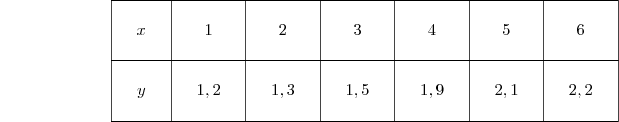
Le gestionnaire d'un supermarché, durant le premier semestre du démarrage de ses activités commerciales, observe l'évolution par mois x de son bénéfice y (en millions de francs CFA).
Les données obtenues sont contenues dans le tableau suivant :
1. Nuage de points associés à cette série statistique.
2. Nous devons établir l'équation (D ) de la droite de régression de y en x par la méthode des moindres carrés.
La droite de régression de y en x est de la forme où et
Notations utilisées :
Tableau statistique complété :
Nous obtenons :
Dès lors,
Par conséquent, l'équation de la droite de régression de y en x est :
3. Représentation graphique de la droite de régression et placement du point moyen G.
4. Nous devons estimer graphiquement le profit au septième mois.
Nous observons sur le graphique que l'ordonnée du point de la droite (D ) d'abscisse 7 est égale à 2,45.
Donc nous pouvons estimer qu'au septième mois suivant le démarrage des activités, le profit du gestionnaire est égal à 2,45 millions de francs CFA.
5. Par le calcul, vérifions si l'estimation de la question précédente est correcte.
Dans l'équation (D), remplaçons x par 7 et calculons la valeur de y .
Par le calcul, nous trouvons que le profit du gestionnaire est égal à 2,46 millions de francs CFA, ce qui rend plausible l'estimation graphique.
5 points
exercice 2
1. Nous savons que deux nombres ont une somme S et un produit P si et seulement si ces nombres sont les solutions de l'équation : x2 - Sx + P = 0.
La somme du deuxième et du quatrième amortissement est 157 537,77 F et leur produit est 6 148 514 623,9.
Ces nombres sont donc les solutions de l'équation :
Les amortissements vérifient donc bien l'équation :
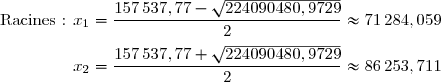
Résolvons l'équation :
Discriminant :
Par conséquent, le deuxième amortissement est égal à 71 284,059 F et le quatrième amortissement est égal à 86 253,711 F.
2. Nous devons déterminer le taux d'intérêt i .
Si u2 représente le montant du deuxième amortissement et u4 représente le montant du quatrième amortissement, nous savons que :
Il s'ensuit que :
Nous en déduisons que le taux d'intérêt est i = 10%.
3. Nous devons déterminer le premier amortissement u1.
Si u2 représente le montant du deuxième amortissement, nous savons que :
Il s'ensuit que :
Par conséquent, le premier amortissement s'élève à 64 803,69 F.
4. Nous devons déterminer le nombre n d'annuités et la dette initiale d sachant que le montant de l'annuité est 114 803,69 F.
Nous savons que le premier amortissement s'élève à 64 803,69 F et que le taux d'intérêt est i = 0,1.
Il s'ensuit que :
D'où il faudra 6 annuités pour rembourser la dette initiale d .
Désignons par un l'amortissement de la nième année.
Dans ce cas,
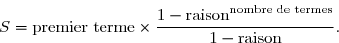
d est donc la somme des 6 premiers termes d'une suite géométrique de raison q = 1,1 dont le premier terme est u1 = 64 803,69.
Or la somme S de termes d'une suite géométrique est donnée par :
Donc
Nous en déduisons que la dette initiale s'élève à 500 000 F.
10 points
probleme
Partie A :
Soit la fonction g définie par :
1. a) Le domaine de définition de g est Dg = .
1. b) Nous devons calculer les limites de g aux bornes de son domaine de définition.
2. a) La fonction g est dérivable sur .
2. b) Nous devons dresser le tableau de variation de g .
L'exponentielle est strictement positive sur .
Donc le signe de g' (x ) est le signe de (2x - 3).
D'où le tableau de variation de g .
3. a)
3. b) Tableau de variations de g complété par le signe de g (x ).
Par conséquent, g(x) > 0 sur l'intervalle ]- ; 0[ g(x) < 0 sur l'intervalle ]0 ; +[.
Partie B :
Soit la fonction f définie par :
1. a) L'ensemble de définition de f est Df = .
1. b) Nous devons calculer les limites de f aux bornes de son ensemble de définition.
Calculons
Il s'ensuit, par produit, que
Par conséquent,
Calculons
Il s'ensuit que
Par conséquent,
1. c) La fonction f est dérivable sur .
1. d) Nous devons dresser le tableau de variation de f .
En utilisant le signe de g(x) étudié dans la partie A, question 3b) et en sachant que nous pouvons dresser le tableau de variation de f .
1. e) Nous devons montrer que l'équation f (x ) = 0 admet deux solutions dans .
Sur l'intervalle
La fonction f est définie, continue et strictement croissante sur l'intervalle et
D'où
Selon le corollaire du théorème des valeurs intermédiaires, nous déduisons que l'équation f (x ) = 0 possède une et une seule solution notée dans l'intervalle
D'où
Sur l'intervalle
La fonction f est définie, continue et strictement décroissante sur l'intervalle et
D'où
Selon le corollaire du théorème des valeurs intermédiaires, nous déduisons que l'équation f (x ) = 0 possède une et une seule solution notée dans l'intervalle
D'où
Par conséquent, l'équation f (x ) = 0 admet deux solutions dans .
1. f) Nous devons montrer que la droite (D ) : y = -x est une asymptote oblique à (Cf ) en +.
Il s'ensuit que la droite (D ) : y = -x est une asymptote oblique à (Cf ) en +
1. g) Nous devons étudier la position relative de (Cf ) par rapport à (D ).
Etudions le signe de f (x ) - (-x ).
Étant donné que l'exponentielle est strictement positive sur , le signe de f (x ) - (-x ) est le signe de (2x + 1).
soit
Nous en déduisons que :
(Cf ) est en dessous de (D ) sur l'intervalle (Cf ) est au-dessus de (D ) sur l'intervalle
1. h) Représentation graphique de (Cf ) et de (D ).
2. Soit h la restriction de f sur ]0 ; +[.
2. a) La fonction h est continue et strictement décroissante sur ]0 ; +[ (voir question 1. d).
Nous savons que h (0) = 1 et
Donc la fonction h est bijective de ]0 ; +[ vers ]- ; 1[.
2. b)
Nous remarquons que
Nous devons en déduire
2. c) Représentation graphique de (Ch-1 ).
Les courbes (Ch-1 ) et (Ch ) sont symétriques par rapport à la droite () : y = x .
D'où la construction de (Ch-1 ).
Publié par malou
le
ceci n'est qu'un extrait
Pour visualiser la totalité des cours vous devez vous inscrire / connecter (GRATUIT) Inscription Gratuitese connecter
Merci à Hiphigenie / malou pour avoir contribué à l'élaboration de cette fiche
Désolé, votre version d'Internet Explorer est plus que périmée ! Merci de le mettre à jour ou de télécharger Firefox ou Google Chrome pour utiliser le site. Votre ordinateur vous remerciera !
 où
où }{V(x)}}) et
et 
=\dfrac{1}{n}\,\sum\limits_{i=1}^n(x_i-\overline{x})(y_i-\overline{y}) \\\\\phantom{WWWWWWWWWWWW}=\dfrac{1}{n}\,\sum\limits_{i=1}^nx_iy_i-\overline{x}\,\overline{y} \\\\ \bullet{\phantom{w}}\text{Variance : }V(x)=\dfrac{1}{n}\,\sum\limits_{i=1}^n(x_i-\overline{x})^2\\\\\phantom{WWWWnWWWWW}=\dfrac{1}{n}\,\sum\limits_{i=1}^nx_i^2-(\overline{x})^2)
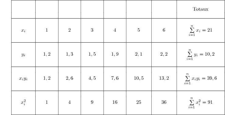
=\dfrac{1}{6}\times39,6-3,5\times1,7=0,65 \\\\ {\phantom{ww}}\bullet{\phantom{w}}\text{Variance : }V(x)=\dfrac{1}{6}\times91-3,5^2=\dfrac{35}{12})
}{V(x)}=\dfrac{0,65}{\frac{35}{12}}=\dfrac{0,65\times12}{35}=\dfrac{7,8}{35}=\dfrac{5\times7,8}{5\times35}=\dfrac{39}{175}\approx0,22\\\\ b=\overline{y}-a\overline{x}=1,7-\dfrac{39}{175}\times3,5=0,92)
:y=0,22x+0,92}\,.)


^2.)
^2=\dfrac{86\,253,711}{71\,284,059}\phantom{w}\Longleftrightarrow\phantom{w}1+i=\sqrt{\dfrac{86\,253,711}{71\,284,059}} \\\\\phantom{(1+i)^2=\dfrac{86\,253,711}{71\,284,059}\phantom{w}}\Longleftrightarrow\phantom{w}i=\sqrt{\dfrac{86\,253,711}{71\,284,059}}-1 \\\\\phantom{(1+i)^2=\dfrac{86\,253,711}{71\,284,059}\phantom{w}}\Longrightarrow\phantom{w}i\approx0,1)
\,u_1.)
\times u_1\phantom{w}\Longleftrightarrow\phantom{w}71\,284,059=1,1\, u_1 \\\\\phantom{71\,284,059=(1+0,1)\times u_1\phantom{w}}\Longleftrightarrow\phantom{w} u_1=\dfrac{71\,284,059}{1,1} \\\\\phantom{71\,284,059=(1+0,1)\times u_1\phantom{w}}\Longleftrightarrow\phantom{w} \boxed{u_1=64\,803,69})
^n.)
^n\Longleftrightarrow114\,803,69=64 803,69\times1,1^n \\\overset{{\white{.}}}{\phantom{\text{Or }\,114\,803,69=64 803,69(1+0,1)^n}\Longleftrightarrow1,1^n=\dfrac{114\,803,69}{64\,803,69}} \\\overset{{\white{.}}}{\phantom{\text{Or }\,114\,803,69=64 803,69(1+0,1)^n}\Longleftrightarrow\ln(1,1^n)=\ln\left(\dfrac{114\,803,69}{64\,803,69}\right)} \\\overset{{\white{.}}}{\phantom{\text{Or }\,114\,803,69=64 803,69(1+0,1)^n}\Longleftrightarrow n\times\ln(1,1)=\ln(114\,803,69)-\ln(64\,803,69)} \\\overset{{\phantom{.}}}{\phantom{\text{Or }\,114\,803,69=64 803,69(1+0,1)^n}\Longleftrightarrow n=\dfrac{\ln(114\,803,69)-\ln(64\,803,69)}{\ln(1,1)}} \\\overset{{\phantom{.}}}{\phantom{\text{Or }\,114\,803,69=64 803,69(1+0,1)^n}\Longrightarrow \boxed{n\approx6}})

^6}{1-1,1}=500\,000.)
=(1-2x)\,\text{e}^{-x}-1.)
 .
.![\\\\\bullet\phantom{w}\left\lbrace\begin{matrix}\lim\limits_{x\to-\infty}(1-2x)=+\infty\phantom{wwwwwwwwwww}\\\\\left\begin{matrix}\lim\limits_{x\to-\infty}(-x)=+\infty\\\\\lim\limits_{X\to+\infty}\text{e}^X=+\infty \end{matrix}\right\rbrace\Longrightarrow\lim\limits_{x\to-\infty}\text{e}^{-x}=+\infty\end{matrix}\right\phantom{w}\Longrightarrow\phantom{w}\lim\limits_{x\to-\infty}(1-2x)\,\text{e}^{-x}=+\infty \\\phantom{WWWWWWWWWWWWWWWWWWiWW}\Longrightarrow\phantom{w}\lim\limits_{x\to-\infty}\left[(1-2x)\,\text{e}^{-x}-1\right]=+\infty \\\\\phantom{WWWWWWWWWWWWWWWWWWiWW}\Longrightarrow\phantom{w}\boxed{\lim\limits_{x\to-\infty}g(x)=+\infty}](https://latex.ilemaths.net/latex-0.tex?\\\\\bullet\phantom{w}\left\lbrace\begin{matrix}\lim\limits_{x\to-\infty}(1-2x)=+\infty\phantom{wwwwwwwwwww}\\\\\left\begin{matrix}\lim\limits_{x\to-\infty}(-x)=+\infty\\\\\lim\limits_{X\to+\infty}\text{e}^X=+\infty \end{matrix}\right\rbrace\Longrightarrow\lim\limits_{x\to-\infty}\text{e}^{-x}=+\infty\end{matrix}\right\phantom{w}\Longrightarrow\phantom{w}\lim\limits_{x\to-\infty}(1-2x)\,\text{e}^{-x}=+\infty \\\phantom{WWWWWWWWWWWWWWWWWWiWW}\Longrightarrow\phantom{w}\lim\limits_{x\to-\infty}\left[(1-2x)\,\text{e}^{-x}-1\right]=+\infty \\\\\phantom{WWWWWWWWWWWWWWWWWWiWW}\Longrightarrow\phantom{w}\boxed{\lim\limits_{x\to-\infty}g(x)=+\infty})
![\bullet\phantom{w}\left\lbrace\begin{matrix}\lim\limits_{x\to+\infty}(1-2x)=-\infty\phantom{wwwwwwwwwww}\\\\\left\begin{matrix}\lim\limits_{x\to+\infty}(-x)=-\infty\\\\\lim\limits_{X\to-\infty}\text{e}^X=0 \end{matrix}\right\rbrace\Longrightarrow\lim\limits_{x\to+\infty}\text{e}^{-x}=0\end{matrix}\right\phantom{w}\Longrightarrow\phantom{w}\begin{matrix}\lim\limits_{x\to+\infty}(1-2x)\,\text{e}^{-x}=0\\ (\text{croissances comparées}) \end{matrix}\\\\\phantom{WWWWWWWWWWWWWWWWWiWW}\Longrightarrow\phantom{w}\lim\limits_ {x\to+\infty}\left[(1-2x)\,\text{e}^{-x}-1\right]=-1 \\\\\phantom{WWWWWWWWWWWWWWWWWiWW}\Longrightarrow\phantom{w}\boxed{\lim\limits_{x\to+\infty}g(x)=-1}](https://latex.ilemaths.net/latex-0.tex?\bullet\phantom{w}\left\lbrace\begin{matrix}\lim\limits_{x\to+\infty}(1-2x)=-\infty\phantom{wwwwwwwwwww}\\\\\left\begin{matrix}\lim\limits_{x\to+\infty}(-x)=-\infty\\\\\lim\limits_{X\to-\infty}\text{e}^X=0 \end{matrix}\right\rbrace\Longrightarrow\lim\limits_{x\to+\infty}\text{e}^{-x}=0\end{matrix}\right\phantom{w}\Longrightarrow\phantom{w}\begin{matrix}\lim\limits_{x\to+\infty}(1-2x)\,\text{e}^{-x}=0\\ (\text{croissances comparées}) \end{matrix}\\\\\phantom{WWWWWWWWWWWWWWWWWiWW}\Longrightarrow\phantom{w}\lim\limits_ {x\to+\infty}\left[(1-2x)\,\text{e}^{-x}-1\right]=-1 \\\\\phantom{WWWWWWWWWWWWWWWWWiWW}\Longrightarrow\phantom{w}\boxed{\lim\limits_{x\to+\infty}g(x)=-1} )
![g'(x)=[(1-2x)\,\text{e}^{-x}]'-1' \\\phantom{g'(x)}=(1-2x)'\times\,\text{e}^{-x}+(1-2x)\times\,(\text{e}^{-x})' \\\phantom{g'(x)}=(-2)\times\,\text{e}^{-x}+(1-2x)\times\,(-x)'\,\text{e}^{-x} \\\phantom{g'(x)}=-2\,\text{e}^{-x}+(1-2x)\times\,(-1)\,\text{e}^{-x} \\\phantom{g'(x)}=-2\,\text{e}^{-x}-(1-2x)\,\text{e}^{-x} \\\phantom{g'(x)}=(-2-1+2x)\,\text{e}^{-x} \\\phantom{g'(x)}=(-3+2x)\,\text{e}^{-x} \\\\\Longrightarrow\boxed{g'(x)=(2x-3)\,\text{e}^{-x}}](https://latex.ilemaths.net/latex-0.tex?g'(x)=[(1-2x)\,\text{e}^{-x}]'-1' \\\phantom{g'(x)}=(1-2x)'\times\,\text{e}^{-x}+(1-2x)\times\,(\text{e}^{-x})' \\\phantom{g'(x)}=(-2)\times\,\text{e}^{-x}+(1-2x)\times\,(-x)'\,\text{e}^{-x} \\\phantom{g'(x)}=-2\,\text{e}^{-x}+(1-2x)\times\,(-1)\,\text{e}^{-x} \\\phantom{g'(x)}=-2\,\text{e}^{-x}-(1-2x)\,\text{e}^{-x} \\\phantom{g'(x)}=(-2-1+2x)\,\text{e}^{-x} \\\phantom{g'(x)}=(-3+2x)\,\text{e}^{-x} \\\\\Longrightarrow\boxed{g'(x)=(2x-3)\,\text{e}^{-x}})
=\left(1-2\times\dfrac{3}{2}\right)\text{e}^{-\frac{3}{2}}-1\\=-2\,\text{e}^{-\frac{3}{2}}-1\phantom{w.}\end{matrix}{\white{www}}\begin{matrix} |\\|\\|\\|\\|\\|\\|\\|\\|\\|\\|\\|\end{matrix}{\white{www}}\begin{matrix} \begin{array}{|c|ccccc|}\hline &&&&&\\ x&-\infty&&\dfrac{3}{2}&&+\infty\\&&&&&\\\hline2x-3&&-&0&+&\\\hline&&&&&\\g\,'(x)&&-&0&+&\\&&&&&\\\hline&+\infty&&&&-1\\g(x)&&\searrow&&\nearrow&\\&&&-2\,\text{e}^{-\frac{3}{2}}-1&&\\ \hline \end{array}\end{matrix})
=(1-2\times0)\,\text{e}^{0}-1=1-1=0\Longrightarrow\boxed{g(0)=0}\,.)
&&\searrow&&0&&\searrow&&\nearrow&\\&&&&&&&-2\,\text{e}^{-\frac{3}{2}}-1&&\\\hline &&&&&&&&&\\g(x)&&+&&0&&-&-&-&\\&&&&&&&&&\\ \hline \end{array})
 g(x) > 0 sur l'intervalle ]-
 ; 0[
; 0[=2x\,\text{e}^{-x}+\text{e}^{-x}-x.)
.})
=2x\,\text{e}^{-x}+\text{e}^{-x}-x \\\phantom{f(x)}=2x\,\text{e}^{-x}+\text{e}^{-x}-x\times1 \\\phantom{f(x)}=2x\,\text{e}^{-x}+\text{e}^{-x}-x\times\text{e}^{-x}\times\text{e}^{x} \\\phantom{f(x)}=-\text{e}^{-x}(-2x-1+x\,\text{e}^{x}) \\\\\Longrightarrow\boxed{f(x)=-\text{e}^{-x}(-2x-1+x\,\text{e}^{x})})
=+\infty\\\\\lim\limits_{X\to+\infty}\text{e}^X=+\infty\end{matrix}\right.\phantom{w}\Longrightarrow\phantom{w}\lim\limits_{x\to-\infty}\text{e}^{-x}=+\infty \\\phantom{WWWWWWWiWWW}\Longrightarrow\phantom{w}\boxed{\lim\limits_{x\to-\infty}-\text{e}^{-x}=-\infty } \\\\\\ \bullet\phantom{w}\left\lbrace\begin{matrix}\lim\limits_{x\to-\infty}(-2x-1)=+\infty\\\\\begin{matrix}\lim\limits_{x\to-\infty}x\,\text{e}^x=0\\ (\text{croissances comparées)} \end{matrix}\end{matrix}\right.\phantom{w}\Longrightarrow\phantom{w}\boxed{\lim\limits_{x\to-\infty}(-2x-1+x\,\text{e}^{x})=+\infty})
=-\infty.})
=-\infty } })
.})
})
=-\infty.})
=-\infty } })
={\red{(2x\,\text{e}^{-x})'}}+(\text{e}^{-x})'-x' \\\phantom{f'(x)}={\red{(2x)'\times\,\text{e}^{-x}+2x\times\,(\text{e}^{-x})'}}+(\text{e}^{-x})'-1 \\\phantom{f'(x)}=2\times\,\text{e}^{-x}+2x\times\,(-\text{e}^{-x})-\text{e}^{-x}-1 \\\phantom{f'(x)}=2\,\text{e}^{-x}-2x\,\text{e}^{-x}-\text{e}^{-x}-1 \\\phantom{f'(x)}=\text{e}^{-x}-2x\,\text{e}^{-x}-1 \\\phantom{f'(x)}=(1-2x)\,\text{e}^{-x}-1 \\\phantom{f'(x)}=g(x) \\\\\Longrightarrow\boxed{f'(x)=g(x)=(1-2x)\,\text{e}^{-x}-1})
=0+\text{e}^{0}-0=1,) nous pouvons dresser le tableau de variation de f .
nous pouvons dresser le tableau de variation de f .&&+&0&-&\\\hline &&&&&\\f'(x)&&+&0&-&\\ &&&&&\\\hline&&&1&&\\f(x)&&\nearrow&&\searrow&\\&-\infty&&&&-\infty\\ \hline \end{array})
 Sur l'intervalle
 ![\overset{{\white{.}}}{]-\infty\,;0[.}](https://latex.ilemaths.net/latex-0.tex?\overset{{\white{.}}}{]-\infty\,;0[.})
=-\infty}) et
et =1.} )
![\overset{{\white{.}}}{ 0\in f(\,]-\infty\,;0[\,).}](https://latex.ilemaths.net/latex-0.tex?\overset{{\white{.}}}{ 0\in f(\,]-\infty\,;0[\,).})
 dans l'intervalle
 \approx-0,105<0 \\\\f(-0,6)\approx0,236>0\end{matrix}\right.)
![\overset{{\white{.}}}{]0\,;\,+\infty[.}](https://latex.ilemaths.net/latex-0.tex?\overset{{\white{.}}}{]0\,;\,+\infty[.})
=1}) et
et =-\infty}.} )
![\overset{{\white{.}}}{ 0\in f(\,]0\,;\,+\infty[\,).}](https://latex.ilemaths.net/latex-0.tex?\overset{{\white{.}}}{ 0\in f(\,]0\,;\,+\infty[\,).})
 dans l'intervalle
 \approx0,104>0 \\\\f(1,1)\approx-0,035<0\end{matrix}\right.)
![\lim\limits_{x\to+\infty}[f(x)-(-x)]=\lim\limits_{x\to+\infty}[(2x\,\text{e}^{-x}+\text{e}^{-x}-x)+x] \\\overset{{\white{.}}}{\phantom{\lim\limits_{x\to+\infty}[f(x)-(-x)]}=\lim\limits_{x\to+\infty}(2x\,\text{e}^{-x}+\text{e}^{-x})} \\\overset{{\white{.}}}{\phantom{\lim\limits_{x\to+\infty}[f(x)-(-x)]}=\lim\limits_{x\to+\infty}2x\,\text{e}^{-x}+\lim\limits_{x\to+\infty}\text{e}^{-x}} \\\overset{{\white{.}}}{\phantom{\lim\limits_{x\to+\infty}[f(x)-(-x)]}=0+0=0} \\\\\Longrightarrow\boxed{\lim\limits_{x\to+\infty}[f(x)-(-x)]=0}](https://latex.ilemaths.net/latex-0.tex?\lim\limits_{x\to+\infty}[f(x)-(-x)]=\lim\limits_{x\to+\infty}[(2x\,\text{e}^{-x}+\text{e}^{-x}-x)+x] \\\overset{{\white{.}}}{\phantom{\lim\limits_{x\to+\infty}[f(x)-(-x)]}=\lim\limits_{x\to+\infty}(2x\,\text{e}^{-x}+\text{e}^{-x})} \\\overset{{\white{.}}}{\phantom{\lim\limits_{x\to+\infty}[f(x)-(-x)]}=\lim\limits_{x\to+\infty}2x\,\text{e}^{-x}+\lim\limits_{x\to+\infty}\text{e}^{-x}} \\\overset{{\white{.}}}{\phantom{\lim\limits_{x\to+\infty}[f(x)-(-x)]}=0+0=0} \\\\\Longrightarrow\boxed{\lim\limits_{x\to+\infty}[f(x)-(-x)]=0})
-(-x)=(2x\,\text{e}^{-x}+\text{e}^{-x}-x)+x \\\overset{{\white{.}}}{\phantom{f(x)-(-x)}=2x\,\text{e}^{-x}+\text{e}^{-x}} \\\overset{{\white{.}}}{\phantom{f(x)-(-x)}=(2x+1)\,\text{e}^{-x}} \\\\\Longrightarrow\boxed{f(x)-(-x)=(2x+1)\,\text{e}^{-x}})
-(-x)<0\Longleftrightarrow x<-\dfrac{1}{2}\\\overset{{\white{.}}}{f(x)-(-x)>0\Longleftrightarrow x>-\dfrac{1}{2}}\end{matrix}\right.)
![]-\infty\,;\,-\dfrac{1}{2}\,[](https://latex.ilemaths.net/latex-0.tex?]-\infty\,;\,-\dfrac{1}{2}\,[)
![]-\dfrac{1}{2}\,;\,+\infty\,[.](https://latex.ilemaths.net/latex-0.tex?]-\dfrac{1}{2}\,;\,+\infty\,[.)
=-\infty.})
=2\,\text{e}^{-1}+\text{e}^{-1}-1\Longrightarrow\boxed{h(1)=3\,\text{e}^{-1}-1}\,.)
=3\,\text{e}^{-1}-1\phantom{ww}\Longleftrightarrow\phantom{ww} h^{-1}(3\,\text{e}^{-1}-1)=1)
'(3\,\text{e}^{-1}-1).)
'(3\,\text{e}^{-1}-1)=\dfrac{1}{h'(h^{-1}(3\,\text{e}^{-1}-1))}=\dfrac{1}{h'(1)}\Longrightarrow\boxed{(h^{-1})'(3\,\text{e}^{-1}-1)=\dfrac{1}{h'(1)}} \\\\\text{Or }h'(1)=g(1)=(1-2\times1)\,\text{e}^{-1}-1\,(\text{voir question 1. c}) \\\\\Longrightarrow \boxed{h'(1)=-\text{e}^{-1}-1} \\\\\text{D'où }\,(h^{-1})'(3\,\text{e}^{-1}-1)=\dfrac{1}{-\text{e}^{-1}-1}\Longleftrightarrow\boxed{(h^{-1})'(3\,\text{e}^{-1}-1)=-\dfrac{1}{\text{e}^{-1}+1}})
 ) : y = x .
 Voir la correction
 forum de terminale