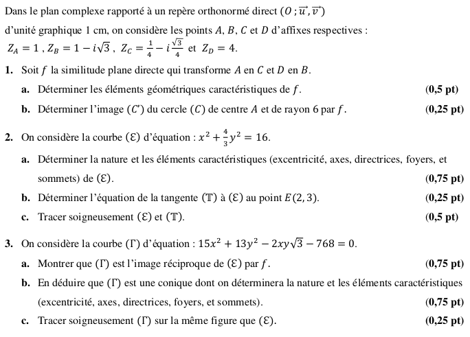
2. b) Déterminons l'équation de la tangente à au point
Nous obtenons :
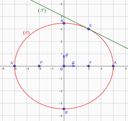
2. c) Représentons graphiquement et
3. On considère la courbe d'équation :
3. a) Montrons que est l'image réciproque de par
Nous avons montré dans la question 1. a) que l'expression algébrique de est
Posons et
Nous obtenons alors :
Soit le point appartenant à l'image réciproque de par
Nous savons alors qu'il existe un point appartenant à tel que
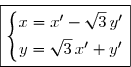
Nous obtenons ainsi le système :
Dans la troisième équation, remplaçons et par leurs valeurs tirées des deux premières équations.
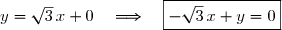
Par conséquent, l'image réciproque de par est la courbe d'équation :
3. b) L'image réciproque de la similitude directe est une similitude directe et l'image d'une ellipse par une similitude directe est une ellipse.
Donc l'image réciproque de l'ellipse par est une ellipse.
Dès lors, est une ellipse.
Déterminons les éléments caractéristiques de sur base des éléments caractéristiques de
Nous avons montré dans la question 3. a) que si appartient à alors il existe un point appartenant
à tel que
Il s'ensuit que :
D'où
Nous pouvons ainsi en déduire les éléments caractéristiques de
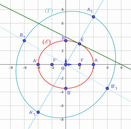
Sommets de : Sommets de notés
Foyers de : Foyers de notés
Excentricité :
Axe focal de : Axe focal de :
Axe non-focal de : Axe non-focal de :
Directrices de : Directrices de :
3. c) Représentons graphiquement
5 points
exercice 2
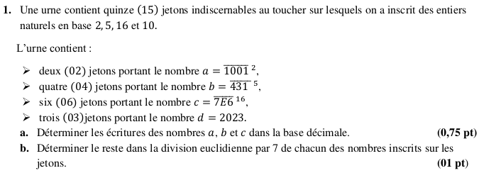
1. Une urne contient 15 jetons.
2 jetons portent le nombre 4 jetons portent le nombre 6 jetons portent le nombre 3 jetons portent le nombre
1. a) Nous devons déterminer les écritures des nombres et dans la base décimale.
1. b) Nous devons déterminer le reste de la division euclidienne par 7 de chacun des nombres inscrits sur les jetons.
2. On pose où est un entier naturel.
2. a) Démontrons que
Par conséquent,
2. b) Déterminons le reste de la division euclidienne de par 7.
En utilisant les informations de la question 2. a), nous obtenons :
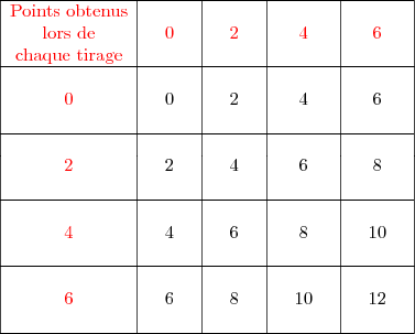
3. L'urne est utilisée dans un jeu.
Le joueur tire un jeton, note le numéro et le remet dans l'urne avant de procéder à un second tirage.
Pour chaque tirage, le joueur gagnera un nombre de points égal au reste de la division euclidienne par 7 du nombre inscrit sur le jeton.
Soit la variable aléatoire associée au nombre de points obtenus par le joueur à l'issue des deux tirages.
3. a) Déterminons la loi de probabilité de
Dans la question 1. b), nous avons montré que les valeurs possibles pour les restes de la division euclidienne par 7 des nombres inscrits sur les jetons étaient 0, 2, 4 et 6.
Notons dans le tableau suivant les diverses manières d'obtenir les différents totaux de points.
Nous en déduisons que les valeurs possibles de la variable sont : 0, 2, 4, 6, 8, 10 et 12.
Nous sommes en situation d'équiprobabilité et les deux tirages sont indépendants.
3 jetons parmi les 15 jetons portent le nombre et attribuent dès lors 0 point.
Lors d'un tirage, la probabilité d'obtenir 0 point est égale à
2 jetons parmi les 15 jetons portent le nombre et attribuent dès lors 2 points.
Lors d'un tirage, la probabilité d'obtenir 2 points est égale à
4 jetons parmi les 15 jetons portent le nombre et attribuent dès lors 4 points.
Lors d'un tirage, la probabilité d'obtenir 4 points est égale à
6 jetons parmi les 15 jetons portent le nombre et attribuent dès lors 6 points.
Lors d'un tirage, la probabilité d'obtenir 6 points est égale à
Calculons
Pour obtenir , nous devons 0 point aux deux tirages.
D'où
Calculons
Pour obtenir , nous devons ''obtenir 2 points au premier tirage et 0 point au second tirage'' ou ''obtenir 0 point au premier tirage et 2 points au second tirage''.
D'où
Calculons
Pour obtenir , nous devons ''obtenir 4 points au premier tirage et 0 point au second tirage'' ou ''obtenir 0 point au premier tirage et 4 points au second tirage'' ou ''obtenir 2 points aux deux tirages''.
D'où
Calculons
Pour obtenir , nous devons ''obtenir 6 points au premier tirage et 0 point au second tirage'' ou ''obtenir 0 point au premier tirage et 6 points au second tirage'' ou ''obtenir 2 points au premier tirage et 4 points au second tirage'' ou ''obtenir 4 points au premier tirage et 2 points au second tirage''.
D'où
Calculons
Pour obtenir , nous devons ''obtenir 2 points au premier tirage et 6 points au second tirage'' ou ''obtenir 6 points au premier tirage et 2 points au second tirage'' ou ''obtenir 4 points aux deux tirages''.
D'où
Calculons
Pour obtenir , nous devons ''obtenir 6 points au premier tirage et 4 points au second tirage'' ou ''obtenir 4 points au premier tirage et 6 points au second tirage''.
D'où
Calculons
Pour obtenir , nous devons 6 points aux deux tirages.
D'où
Résumons cette loi de probabilité de par le tableau suivant :
3. b) Calculons l'espérance mathématique
3. c) Calculons la probabilité d'avoir un gain dépassant l'espérance, soit
11 points
probleme
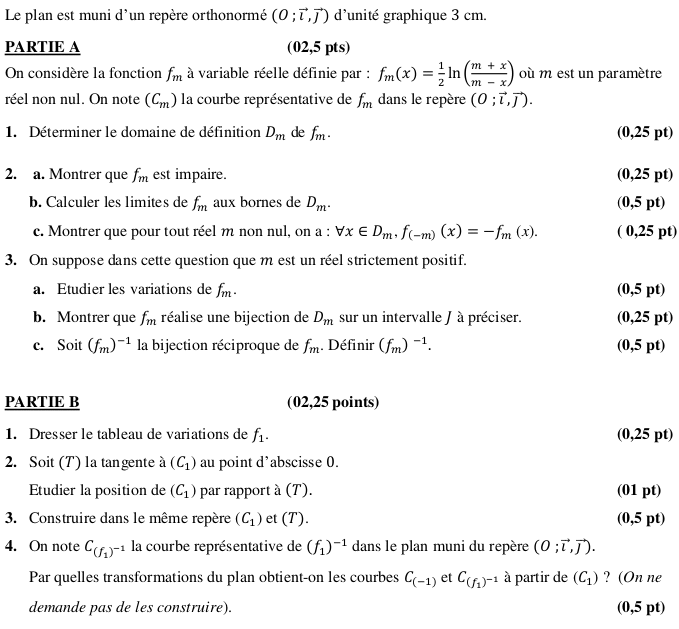
Le plan est muni d'un repère orthonormé
Partie A (2,5 points)
On considère la fonction à variable réelle définie par : où est un paramètre réel non nul.
On note la courbe représentative de dans la repère
1. Déterminons le domaine de définition de
Envisageons deux cas.
Premier cas :
D'où si alors
Second cas :
D'où si alors
Par conséquent,
2. a) Montrons que est impaire.
Nous en déduisons que est impaire.
2. b) Nous devons calculer les limites de aux bornes de
Envisageons deux cas.
Premier cas : (nous savons que dans ce cas, )
Calculons
D'où
Calculons
D'où
Second cas : (nous savons que dans ce cas, )
Calculons
D'où
Calculons
D'où
2. c) Montrons que pour tout réel non nul, nous avons :
3. On suppose dans cette question que est un réel strictement positif.
3. a) Nous devons étudier les variations de
La fonction est dérivable sur
Donc
Par conséquent, la fonction est strictement croissante sur
3. b) La fonction est continue et strictement croissante sur
Dès lors, réalise une bijection de sur
3. c) Soit la bijection réciproque de
Nous pouvons ainsi définir comme suit :
où le domaine de définition est et l'image est
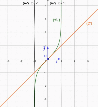
Partie B (2,25 points)
1. Nous devons dresser le tableau de variations de
Nous rappelons que la fonction est définie par :
Nous notons la courbe représentative de dans la repère
En utilisant les résultats de la partie A où , nous obtenons le tableau de variations de
2. Soit la tangente à au point d'abscisse 0.
Déterminons une équation de
Une équation de est de la forme soit
Or
Nous en déduisons qu'une équation de est
Nous déterminerons la position de par rapport à en
étudiant le signe de la fonction définie sur par
La fonction est dérivable sur .
Nous en déduisons que
et par suite la fonction est croissante sur
En outre,
Il s'ensuit que :
soit que
Par conséquent, est en dessous de sur l'intervalle est au-dessus de sur l'intervalle
3. Construisons et
4. Nous avons montré dans la partie A, question 2. c) que pour tout réel non nul, nous avons :
Dès lors,
Par conséquent, la courbe est l'image de la courbe par la symétrie axiale dont l'axe est la droite
De plus, nous savons que si deux fonctions sont réciproques l'une de l'autre, leurs représentations graphiques dans un plan muni d'un repère orthonormé sont symétriques l'une de l'autre par rapport à la droite d'équation
D'où la courbe est l'image de la courbe par la symétrie axiale dont l'axe est la droite
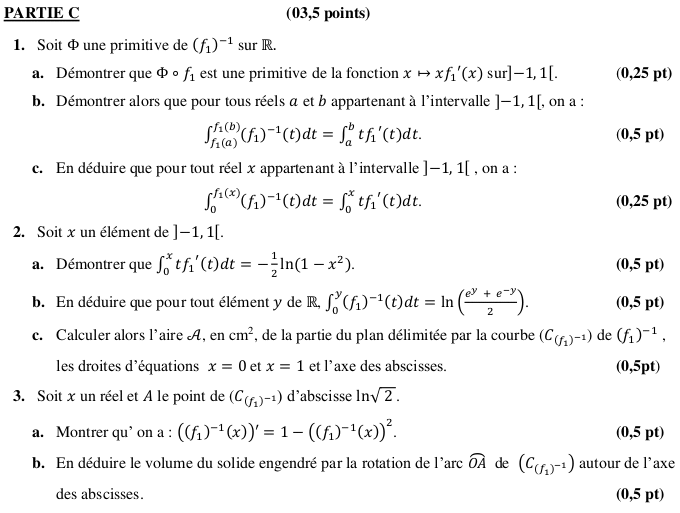
Partie C (3,5 points)
1. Soit une primitive de sur
1. a) Nous devons démontrer que est une primitive de la fonction sur
D'une part, car est une primitive de sur
D'autre part, la fonction est dérivable sur (car est dérivable sur et est dérivable sur ).
Nous obtenons ainsi :
Par conséquent, est une primitive de la fonction
1. b) Nous devons démontrer que pour tous réels et appartenant à l'intervalle on a :
En effet, pour tous réels et appartenant à l'intervalle nous obtenons :
1. c) Nous devons en déduire que pour tout appartenant à l'intervalle nous avons :
Nous savons que
Dès lors, en remplaçant par 0 et par dans l'égalité de la question précédente, nous obtenons :
, soit
2. Soit un élément de
2. a) Démontrons que
Nous avons montré dans la partie A, question 3. a) que et par suite,
Nous obtenons ainsi :
2. b) Nous devons montrer que pour tout élément de
Nous avons montré dans les questions 1. c) et 2. a) que pour tout appartenant à l'intervalle nous avons :
et
Nous en déduisons que
et si alors l'égalité précédente s'écrira :
Dans ce cas, nous savons par la question 3. c) - Partie A que
Dès lors,
2. c) Calculons l'aire , en cm2, de la partie du plan délimitée par la courbe
, les droites d'équations et et l'axe des abscisses.
Déterminons d'abord l'aire en unité d'aire (u.a.) en utilisant le résultat de la question précédente dans lequel nous remplaçons par 1.
Or l'unité graphique du repère est de 3 cm.
Dès lors l'unité d'aire est 9 cm2.
Par conséquent,
3. Soit un réel et le point de d'abscisse
3. a) Montrons que :
En utilisant la définition de donnée dans la Partie A - question 3. c), nous savons que
D'une part, nous obtenons :
D'autre part,
Par conséquent
3. b) Nous devons en déduire le volume du solide engendré par la rotation de l'arc de autour de l'axe des abscisses.
Nous avons :
Or selon la question précédente, nous savons que , soit que
Dès lors,
D'où
Or l'unité graphique est 3 cm.
Donc l'unité de volume (u. v.) est 27 cm3.
Par conséquent,
Partie D (2,75 points)
Soit un nombre réel.
Pour tout entier naturel non nul, on pose :
1. a) Montrons que nous avons :
Nous savons par la question 1 - Partie B que la fonction est strictement croissante sur
Dès lors, la fonction est strictement croissante sur
Nous obtenons alors :
1. b) Nous devons en déduire pour tout réel positif fixé, la limite de
Nous savons par la question 3. c) - Partie A que
Nous obtenons alors :
De plus, nous avons montré dans la question précédente que
Dès lors, en appliquant le théorème d'encadrement (théorème des gendarmes), nous avons pour tout réel positif fixé,
2. a) Montrons que :
En effet, pour tout
2. b) Démontrons par récurrence que :
Initialisation : Montrons que la propriété est vraie pour soit que
Notons d'abord que
De plus,
Donc l'initialisation est vraie.
Hérédité : Montrons que si pour un nombre naturel non nul fixé, la propriété est vraie au rang alors elle est encore vraie au rang
Montrons donc que si pour un nombre naturel non nul fixé, , alors nous obtenons
Donc l'hérédité est vraie.
Puisque l'initialisation et l'hérédité sont vraies, nous avons montré par récurrence que :
3. a) Montrons que pour tout réel appartenant à [0 ; 1[ et pour tout entier naturel non nul nous avons :
En utilisant le résultat de la question 2. b), nous déduisons que pour tout réel appartenant à [0 ; 1[ et pour tout entier naturel non nul nous obtenons :
3. b) Nous devons en déduire :
Nous avons montré dans la question précédente que pour tout réel appartenant à [0 ; 1[ et pour tout entier naturel non nul nous avons :
Remplaçons par nous obtenons ainsi :
De plus, nous savons par la question 1. b) que pour tout réel positif fixé,
Nous en déduisons que pour
Par conséquent, soit
Publié par malou
le
ceci n'est qu'un extrait
Pour visualiser la totalité des cours vous devez vous inscrire / connecter (GRATUIT) Inscription Gratuitese connecter
Merci à Hiphigenie / malou pour avoir contribué à l'élaboration de cette fiche
Désolé, votre version d'Internet Explorer est plus que périmée ! Merci de le mettre à jour ou de télécharger Firefox ou Google Chrome pour utiliser le site. Votre ordinateur vous remerciera !

}) d'unité graphique 1 cm,
on considère les points
d'unité graphique 1 cm,
on considère les points  et
et  d'affixes respectives :
 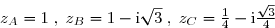 et
et 
 la similitude plane directe qui transforme
  en
en  et
et 


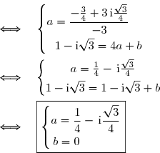
=C\\f(D)=B\end{matrix}\right.\quad\Longleftrightarrow\quad \left\lbrace\begin{matrix}z_C=az_A+b\\z_B=az_D+b\end{matrix}\right. \\\overset{ { \white{ . } } } { \phantom{WWWWW}\quad\Longleftrightarrow\quad \left\lbrace\begin{matrix}z_C-z_B=(az_A+b)-(az_D+b)\\z_B=az_D+b\phantom{WWWWWWWW}\end{matrix}\right.} \\\overset{ { \white{ . } } } { \phantom{WWWWW}\quad\Longleftrightarrow\quad \left\lbrace\begin{matrix}z_C-z_B=az_A-az_D\\z_B=az_D+b\phantom{WWW}\end{matrix}\right.} \\\overset{ { \white{ . } } } { \phantom{WWWWW}\quad\Longleftrightarrow\quad \left\lbrace\begin{matrix}z_C-z_B=a(z_A-z_D)\\z_B=az_D+b\phantom{WWW}\end{matrix}\right.})

-(1-\text i\sqrt 3)}{1-4}\\\overset{ { \phantom{ . } } } {1-\text i\sqrt 3=a\times4+b}\phantom{WWW}\end{matrix}\right.} \\\overset{ { \white{ . } } } { \phantom{WWWWW}\quad\Longleftrightarrow\quad \left\lbrace\begin{matrix}a=\dfrac{\frac 1 4-\text i\frac{\sqrt 3}{4}-1+\text i\sqrt 3}{-3}\\\overset{ { \phantom{ . } } } {1-\text i\sqrt 3=4a+b}\phantom{W}\end{matrix}\right.})
z}\,. })
 Le centre de


^2+\left( \dfrac{\sqrt 3}{4}\right)^2}=\sqrt{\dfrac {1} {16}+ \dfrac{3}{16}}=\sqrt{\dfrac {4} {16}}=\sqrt{\dfrac {1} {4}}=\dfrac12})

![\theta=\arg\left(\dfrac 1 4-\,\text i\dfrac{\sqrt 3}{4}\right) \\\\\text{Or }\left\lbrace\begin{matrix}\cos\theta=\dfrac{\frac 1 4}{\left|\frac 1 4-\,\text i\frac{\sqrt 3}{4}\right|}=\dfrac{\frac 1 4}{\frac1 2}=\dfrac 12\phantom{xx}\\\overset{ { \white{ . } } } {\sin\theta=\dfrac{-\frac{\sqrt 3}{4}}{\frac1 2}=-\dfrac{\sqrt3}{2}\phantom{WWWx}}\end{matrix}\right.\quad\Longrightarrow\quad \theta=-\dfrac{\pi}{3}\,[2\pi]](https://latex.ilemaths.net/latex-0.tex?\theta=\arg\left(\dfrac 1 4-\,\text i\dfrac{\sqrt 3}{4}\right) \\\\\text{Or }\left\lbrace\begin{matrix}\cos\theta=\dfrac{\frac 1 4}{\left|\frac 1 4-\,\text i\frac{\sqrt 3}{4}\right|}=\dfrac{\frac 1 4}{\frac1 2}=\dfrac 12\phantom{xx}\\\overset{ { \white{ . } } } {\sin\theta=\dfrac{-\frac{\sqrt 3}{4}}{\frac1 2}=-\dfrac{\sqrt3}{2}\phantom{WWWx}}\end{matrix}\right.\quad\Longrightarrow\quad \theta=-\dfrac{\pi}{3}\,[2\pi])
 , son rapport est
  et son angle est
 }) du cercle
du cercle  }) de centre
de centre 
=C }) dont le rayon est
dont le rayon est 
 }) d'équation
d'équation 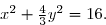
. })
^2}=1} \\\overset{ { \white{ . } } } {\phantom{WWWWWW}\quad\Longleftrightarrow\quad \boxed{\dfrac{x^2}{4^2}+\dfrac {y^2}{(2\sqrt{3})^2}=1}})

: })
,\,A'\,(-4\;;\;0),\,B\,(0\;;\;2\sqrt 3)\;\text{ et }\;B'\,(0\;;\;-2\sqrt 3). })
\;\text{ et }\;F'\,(-2\;;\;0). })


:x=\dfrac{a^2}{c}=\dfrac{16}{2}\phantom{WW}\\\overset{ { \white{ . } } } { (D'):x=-\dfrac{a^2}{c}=-\dfrac{16}{2}}\end{matrix}\right.\quad\Longrightarrow\quad \left\lbrace\begin{matrix}(D):x=8\phantom{x}\\\overset{ { \white{ . } } } { (D'):x=-8}\end{matrix}\right. })
 }) à
à  })
:x\times2+\dfrac 4 3 y\times3=16\quad\Longleftrightarrow\quad(\mathscr{T}):2x+4y=16 \\\phantom{xxx:x\times2+\dfrac 4 3 y\times3=16}\quad\Longleftrightarrow\quad(\mathscr{T}):x+2y=8)

 :x+2y-8=0})
. })
 }) d'équation :
d'équation : 
 et
et 
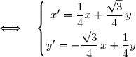
z\quad\Longleftrightarrow\quad x'+\text i\,y'= \left(\dfrac 1 4-\,\text i\,\dfrac{\sqrt 3}{4}\right)(x+\text i\,y) \\\phantom{WWWWWWWw}\quad\Longleftrightarrow\quad x'+\text i\,y'= \left(\dfrac 1 4-\,\text i\,\dfrac{\sqrt 3}{4}\right)x+\text i\left(\dfrac 1 4-\,\text i\,\dfrac{\sqrt 3}{4}\right)\,y \\\phantom{WWWWWWWw}\quad\Longleftrightarrow\quad x'+\text i\,y'=\dfrac 1 4x-\,\text i\,\dfrac{\sqrt 3}{4}x+\dfrac 1 4\,\text i\,y+\dfrac{\sqrt 3}{4}\,y \\\phantom{WWWWWWWw}\quad\Longleftrightarrow\quad x'+\text i\,y'=\left(\dfrac 1 4x+\dfrac{\sqrt 3}{4}\,y\right)+\,\text i\,\left(-\dfrac{\sqrt 3}{4}x+\dfrac 1 4\,y\right))

 }) appartenant à l'image réciproque de
appartenant à l'image réciproque de  }) appartenant à
appartenant à  }) tel que
tel que . })

 et
et  par leurs valeurs tirées des deux premières équations.
^2+\dfrac 4 3 \left(-\dfrac{\sqrt 3}{4}\,x+\dfrac 1 4\,y\right)^2=16 \\\\\phantom{XXXXX}\Longleftrightarrow\quad\dfrac{1}{16}x^2+\dfrac{\sqrt3}{8}\,xy+\dfrac{3}{16}y^2+\dfrac 4 3 \left(\dfrac{3}{16}x^2-\dfrac{\sqrt3}{8}xy+\dfrac{1}{16}y^2\right)=16 \\\\\phantom{XXXXX}\Longleftrightarrow\quad\dfrac{1}{16}x^2+\dfrac{\sqrt3}{8}\,xy+\dfrac{3}{16}y^2+\dfrac{1}{4}x^2-\dfrac{\sqrt3}{6}xy+\dfrac{1}{12}y^2=16 \\\\\phantom{XXXXX}\Longleftrightarrow\quad\dfrac{5}{16}x^2+\dfrac{13}{48}y^2-\dfrac{\sqrt3}{24}xy=16 \\\\\phantom{XXXXX}\Longleftrightarrow\quad\dfrac{15}{48}x^2+\dfrac{13}{48}y^2-\dfrac{2\sqrt3}{48}\,xy=16 \\\\\phantom{XXXXX}\Longleftrightarrow\quad15x^2+13y^2-2\sqrt3\,xy=768)
. })
, }) alors il existe un point
alors il existe un point 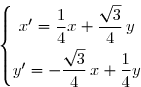
\\\overset{ { \white{ . } } } {-\sqrt 3\,x+y=4y'\quad\quad(2)}\end{matrix}\right.)
\\ (2)\phantom{xxxx}\end{matrix}\right.\quad\Longleftrightarrow\quad \left\lbrace\begin{matrix}\sqrt 3\,x+3y=4\sqrt3\,x'\quad\quad\phantom{x}(3)\\\overset{ { \white{ . } } } {-\sqrt 3\,x+y=4y'\phantom{xxi}\quad\quad(2)}\end{matrix}\right. \\\\ (3)+(2)\quad\Longleftrightarrow\quad 4y=4\sqrt3\,x'+4y' \\\overset{ { \white{ . } } } {\phantom{WWxW}\quad\Longleftrightarrow\quad \boxed{y=\sqrt3\,x'+y'}})
\phantom{xxxxxx}\\\overset{ { \white{ . } } } {-\sqrt 3\times(2)}\end{matrix}\right.\quad\Longleftrightarrow\quad \left\lbrace\begin{matrix}x+\sqrt 3\,y=4x'\quad\quad\phantom{xxxxxxx}(1)\\\overset{ { \white{ . } } } {3x-\sqrt 3\,y=-4\sqrt 3\,y'\phantom{xxi}\quad\quad(4)}\end{matrix}\right. \\\\\phantom{xxx}(1)+(4)\quad\Longleftrightarrow\quad 4x=4x'-4\sqrt3\,y' \\\overset{ { \white{ . } } } {\phantom{WWWWW}\quad\Longleftrightarrow\quad \boxed{x=x'-\sqrt3\,y'}})
. })
 Sommets de
})
+0}\end{matrix}\right. } \quad\Longrightarrow\quad \overset{ { \white{ . } } } { \left\lbrace\begin{matrix}x_{A'_1}=-4\phantom{xx}\\\overset{ { \phantom{ . } } } { y_{A'_1}=-4\sqrt3}\end{matrix}\right. } \quad\Longrightarrow\quad \boxed{A'_1\,(-4\;;\;-4\sqrt 3)})
})
\\\overset{ { \phantom{ . } } } { y_{B'_1}=\sqrt3\times0-2\sqrt 3}\end{matrix}\right. } \quad\Longrightarrow\quad \overset{ { \white{ . } } } { \left\lbrace\begin{matrix}x_{B'_1}=6\phantom{xx}\\\overset{ { \phantom{ . } } } { y_{B'_1}=-2\sqrt3}\end{matrix}\right. } \quad\Longrightarrow\quad \boxed{B'_1\,(6\;;\;-2\sqrt 3)})

})
+0}\end{matrix}\right. } \quad\Longrightarrow\quad \overset{ { \white{ . } } } { \left\lbrace\begin{matrix}x_{F'_1}=-2\phantom{xx}\\\overset{ { \phantom{ . } } } { y_{F'_1}=-2\sqrt3}\end{matrix}\right. } \quad\Longrightarrow\quad \boxed{F'_1\,(-2\;;\;-2\sqrt 3)})

:x=8\phantom{x}\\\overset{ { \white{ . } } } { (D'):x=-8}\end{matrix}\right. )
:\dfrac 1 4x+\dfrac{\sqrt 3}{4}\,y=8\quad\Longrightarrow\quad \boxed{x+\sqrt 3\,y=32}\phantom{i}\\\overset{ { \white{ . } } } { (D'_1):\dfrac 1 4x+\dfrac{\sqrt 3}{4}\,y=-8\quad\Longrightarrow\quad \boxed{x+\sqrt 3\,y=-32}}\end{matrix}\right.})


 et
et  dans la base décimale.
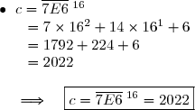
![\overset{ { \white{ . } } }{\bullet}{\white{xx}}a=9=1\times7+2\quad\Longrightarrow\quad\boxed{a\equiv 2\,[7]} \\\overset{ { \phantom{ Z } } }{\bullet}{\phantom{xx}}b=116=16\times7+4\quad\Longrightarrow\quad\boxed{b\equiv 4\,[7]} \\\overset{ { \phantom{Z } } }{\bullet}{\phantom{xx}}c=2022=288\times7+6\quad\Longrightarrow\quad\boxed{c\equiv 6\,[7]} \\\overset{ { \phantom{Z } } }{\bullet}{\phantom{xx}}d=2023=289\times7+0\quad\Longrightarrow\quad\boxed{d\equiv 0\,[7]}](https://latex.ilemaths.net/latex-0.tex?\overset{ { \white{ . } } }{\bullet}{\white{xx}}a=9=1\times7+2\quad\Longrightarrow\quad\boxed{a\equiv 2\,[7]} \\\overset{ { \phantom{ Z } } }{\bullet}{\phantom{xx}}b=116=16\times7+4\quad\Longrightarrow\quad\boxed{b\equiv 4\,[7]} \\\overset{ { \phantom{Z } } }{\bullet}{\phantom{xx}}c=2022=288\times7+6\quad\Longrightarrow\quad\boxed{c\equiv 6\,[7]} \\\overset{ { \phantom{Z } } }{\bullet}{\phantom{xx}}d=2023=289\times7+0\quad\Longrightarrow\quad\boxed{d\equiv 0\,[7]})
 où
où  est un entier naturel.
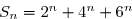
![\overset{ { \white{ . } } } { S_{6n}\equiv3\,[7]. }](https://latex.ilemaths.net/latex-0.tex?\overset{ { \white{ . } } } { S_{6n}\equiv3\,[7]. })
![\text{Or }\;\overset{ { \white{ . } } }{\bullet}{\phantom{x}} 2^6=64=9\times7+1\quad\Longrightarrow\quad2^6\equiv1\,[7]\\\phantom{WWWWWWWWWWW}\quad\Longrightarrow\quad\left(2^6\right)^n\overset{ { \white{ . } } } {\equiv1^n\,[7]} \\\phantom{WWWWWWWWWWW}\quad\Longrightarrow\quad2^{6n}\overset{ { \white{ . } } } {\equiv1\,[7]} \\\\\phantom{xxx}\overset{ { \phantom{ . } } }{\bullet}{\phantom{x}} 4^6=2^6\times2^6\equiv1\times1\,[7]\quad\Longrightarrow\quad4^6\equiv1\,[7]\\\phantom{WWWWWWWWWxWWW}\quad\Longrightarrow\quad\left(4^6\right)^n\overset{ { \phantom{ . } } } {\equiv1^n\,[7]} \\\phantom{WWWWWWWWWWxWW}\quad\Longrightarrow\quad4^{6n}\overset{ { \phantom{ . } } } {\equiv1\,[7]}](https://latex.ilemaths.net/latex-0.tex?\text{Or }\;\overset{ { \white{ . } } }{\bullet}{\phantom{x}} 2^6=64=9\times7+1\quad\Longrightarrow\quad2^6\equiv1\,[7]\\\phantom{WWWWWWWWWWW}\quad\Longrightarrow\quad\left(2^6\right)^n\overset{ { \white{ . } } } {\equiv1^n\,[7]} \\\phantom{WWWWWWWWWWW}\quad\Longrightarrow\quad2^{6n}\overset{ { \white{ . } } } {\equiv1\,[7]} \\\\\phantom{xxx}\overset{ { \phantom{ . } } }{\bullet}{\phantom{x}} 4^6=2^6\times2^6\equiv1\times1\,[7]\quad\Longrightarrow\quad4^6\equiv1\,[7]\\\phantom{WWWWWWWWWxWWW}\quad\Longrightarrow\quad\left(4^6\right)^n\overset{ { \phantom{ . } } } {\equiv1^n\,[7]} \\\phantom{WWWWWWWWWWxWW}\quad\Longrightarrow\quad4^{6n}\overset{ { \phantom{ . } } } {\equiv1\,[7]})
![\\\\\phantom{xxx}\overset{ { \phantom{ . } } }{\bullet}{\phantom{x}} 6^6=2^6\times3^6=2^6\times(3^2)^3\equiv1\times2^3\,[7]\equiv1\times1\,[7]\quad\Longrightarrow\quad6^6\equiv1\,[7]\\\phantom{WWW WWWWWWWWWWWWWWxWWWWW}\quad\Longrightarrow\quad\left(6^6\right)^n\overset{ { \phantom{ . } } } {\equiv1^n\,[7]} \\\phantom{WWWWWWWWWWxWWWWWWWWWWWW}\quad\Longrightarrow\quad6^{6n}\overset{ { \phantom{ . } } } {\equiv1\,[7]} \\\\\Longrightarrow\quad S_{6n}\equiv1+1+1\;[7]](https://latex.ilemaths.net/latex-0.tex?\\\\\phantom{xxx}\overset{ { \phantom{ . } } }{\bullet}{\phantom{x}} 6^6=2^6\times3^6=2^6\times(3^2)^3\equiv1\times2^3\,[7]\equiv1\times1\,[7]\quad\Longrightarrow\quad6^6\equiv1\,[7]\\\phantom{WWW WWWWWWWWWWWWWWxWWWWW}\quad\Longrightarrow\quad\left(6^6\right)^n\overset{ { \phantom{ . } } } {\equiv1^n\,[7]} \\\phantom{WWWWWWWWWWxWWWWWWWWWWWW}\quad\Longrightarrow\quad6^{6n}\overset{ { \phantom{ . } } } {\equiv1\,[7]} \\\\\Longrightarrow\quad S_{6n}\equiv1+1+1\;[7])
![\overset{ { \white{ . } } } { \boxed{S_{6n}\equiv3\,[7]}\,. }](https://latex.ilemaths.net/latex-0.tex?\overset{ { \white{ . } } } { \boxed{S_{6n}\equiv3\,[7]}\,. })
 par 7.
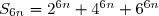
![S_{2023}=2^{2023}+4^{2023}+6^{2023} \\\overset{ { \white{ . } } } {\phantom{S_{2023}}=2\times2^{2022}+4\times4^{2022}+6\times6^{2022}} \\\overset{ { \phantom{ . } } } {\phantom{S_{2023}}=2\times2^{6\times337}+4\times4^{6\times337}+6\times6^{6\times337}} \\\overset{ { \white{ . } } } {\phantom{S_{2023}}\equiv2\times1+4\times1+6\times1\,[7]} \\\overset{ { \white{ . } } } {\phantom{S_{2023}}\equiv12\,[7]} \\\overset{ { \phantom{ . } } } {\phantom{S_{2023}}\equiv5\,[7]} \\\\\Longrightarrow\quad\boxed{S_{2023}\equiv5\,[7]}](https://latex.ilemaths.net/latex-0.tex?S_{2023}=2^{2023}+4^{2023}+6^{2023} \\\overset{ { \white{ . } } } {\phantom{S_{2023}}=2\times2^{2022}+4\times4^{2022}+6\times6^{2022}} \\\overset{ { \phantom{ . } } } {\phantom{S_{2023}}=2\times2^{6\times337}+4\times4^{6\times337}+6\times6^{6\times337}} \\\overset{ { \white{ . } } } {\phantom{S_{2023}}\equiv2\times1+4\times1+6\times1\,[7]} \\\overset{ { \white{ . } } } {\phantom{S_{2023}}\equiv12\,[7]} \\\overset{ { \phantom{ . } } } {\phantom{S_{2023}}\equiv5\,[7]} \\\\\Longrightarrow\quad\boxed{S_{2023}\equiv5\,[7]})
 la variable aléatoire associée au nombre de points obtenus par le joueur à l'issue des deux tirages.

 et attribuent dès lors 0 point.
 et attribuent dès lors 2 points.
 et attribuent dès lors 4 points.
 et attribuent dès lors 6 points.
 Calculons
 . })
 , nous devons 0 point aux deux tirages.
=\dfrac{3}{15}\times\dfrac{3}{15}=\dfrac{9}{225}. })
. })
 , nous devons ''obtenir 2 points au premier tirage et 0 point au second tirage'' ou ''obtenir 0 point au premier tirage et 2 points au second tirage''.
=\dfrac{2}{15}\times\dfrac{3}{15}+\dfrac{3}{15}\times\dfrac{2}{15}=\dfrac{12}{225}. })
. })
 , nous devons ''obtenir 4 points au premier tirage et 0 point au second tirage'' ou ''obtenir 0 point au premier tirage et 4 points au second tirage'' ou ''obtenir 2 points aux deux tirages''.
=\dfrac{4}{15}\times\dfrac{3}{15}+\dfrac{3}{15}\times\dfrac{4}{15}+\dfrac{2}{15}\times\dfrac{2}{15}=\dfrac{28}{225}. })
. })
 , nous devons ''obtenir 6 points au premier tirage et 0 point au second tirage'' ou ''obtenir 0 point au premier tirage et 6 points au second tirage'' ou ''obtenir 2 points au premier tirage et 4 points au second tirage'' ou ''obtenir 4 points au premier tirage et 2 points au second tirage''.
=\dfrac{6}{15}\times\dfrac{3}{15}+\dfrac{3}{15}\times\dfrac{6}{15}+\dfrac{2}{15}\times\dfrac{4}{15}+\dfrac{4}{15}\times\dfrac{2}{15}=\dfrac{52}{225}. })
. })
 , nous devons ''obtenir 2 points au premier tirage et 6 points au second tirage'' ou ''obtenir 6 points au premier tirage et 2 points au second tirage'' ou ''obtenir 4 points aux deux tirages''.
=\dfrac{2}{15}\times\dfrac{6}{15}+\dfrac{6}{15}\times\dfrac{2}{15}+\dfrac{4}{15}\times\dfrac{4}{15}=\dfrac{40}{225}. })
. })
 , nous devons ''obtenir 6 points au premier tirage et 4 points au second tirage'' ou ''obtenir 4 points au premier tirage et 6 points au second tirage''.
=\dfrac{6}{15}\times\dfrac{4}{15}+\dfrac{4}{15}\times\dfrac{6}{15}=\dfrac{48}{225}. })
. })
 , nous devons 6 points aux deux tirages.
=\dfrac{6}{15}\times\dfrac{6}{15}=\dfrac{36}{225}. })
&&\dfrac{9}{225}&&&\dfrac{12}{225}&&&\dfrac{28}{225}&&&\dfrac{52}{225}&&&\dfrac{40}{225}&&&\dfrac{48}{225}&&&\dfrac{36}{225}&\\&&&&&&&&&&&&&&&&&&&&&\\\hline \end{array} )
. })
=0\times\dfrac{9}{225}+2\times\dfrac{12}{225}+4\times\dfrac{28}{225}+6\times\dfrac{52}{225}+8\times\dfrac{40}{225}+10\times\dfrac{48}{225}+12\times\dfrac{36}{225} \\\\\phantom{E(X)}=\dfrac{1680}{225}=\dfrac{112}{15} \\\\\Longrightarrow\quad\boxed{E(X)=\dfrac{112}{15}\approx7,47})
. })
=P(X=8)+P(X=10)+P(X=12) \\\phantom{P\left(X>\dfrac{112}{15}\right)}=\dfrac{40}{225}+\dfrac{48}{225}+\dfrac{26}{225} \\\overset{ { \white{ . } } } {\phantom{P\left(X>\dfrac{112}{15}\right)}=\dfrac{124}{225}} \\\\\Longrightarrow\quad\boxed{P\left(X>\dfrac{112}{15}\right)=\dfrac{124}{225}\approx0,56})
. })
 à variable réelle définie par :
 =\dfrac{1}{2}\,\ln\left(\dfrac{m+x}{m-x}\right) }) où
où  est un paramètre réel non nul.
 }) la courbe représentative de
la courbe représentative de  de
de 

![\begin{matrix}m+x<0\Longleftrightarrow x<-m \\\overset{ { \white{ . } } } {m+x=0\Longleftrightarrow x=-m} \\\overset{ { \phantom{ . } } } {m+x>0\Longleftrightarrow x>-m}\\\\m-x<0\Longleftrightarrow x>m \\\overset{ { \phantom{ . } } } {m-x=0\Longleftrightarrow x=m} \\\overset{ { \phantom{ . } } } {m-x>0\Longleftrightarrow x<m} \end{matrix} \begin{matrix}\\||\\||\\||\\||\\||\\||\\||\\||\\||\\||\\\phantom{WWW}\end{matrix} \begin{array}{|c|ccccccc|}\hline &&&&&&&&x&-\infty&&-m&&m&&+\infty &&&&&&&&\\\hline &&&&&&&\\ m+x&&-&0&+&+&+&\\m-x&&+&+&+&0&-&\\&&&&&&&\\\hline&&&&&||&&\\\dfrac{m+x}{m-x}&&-&0&+&||&-&\\&&&&&||&&\\\hline \end{array} \\\\\text{Donc }\;\dfrac{m+x}{m-x}>0\quad\Longleftrightarrow\quad x\in\;]-m\;;\;m[](https://latex.ilemaths.net/latex-0.tex?\begin{matrix}m+x<0\Longleftrightarrow x<-m \\\overset{ { \white{ . } } } {m+x=0\Longleftrightarrow x=-m} \\\overset{ { \phantom{ . } } } {m+x>0\Longleftrightarrow x>-m}\\\\m-x<0\Longleftrightarrow x>m \\\overset{ { \phantom{ . } } } {m-x=0\Longleftrightarrow x=m} \\\overset{ { \phantom{ . } } } {m-x>0\Longleftrightarrow x<m} \end{matrix} \begin{matrix}\\||\\||\\||\\||\\||\\||\\||\\||\\||\\||\\\phantom{WWW}\end{matrix} \begin{array}{|c|ccccccc|}\hline &&&&&&&&x&-\infty&&-m&&m&&+\infty &&&&&&&&\\\hline &&&&&&&\\ m+x&&-&0&+&+&+&\\m-x&&+&+&+&0&-&\\&&&&&&&\\\hline&&&&&||&&\\\dfrac{m+x}{m-x}&&-&0&+&||&-&\\&&&&&||&&\\\hline \end{array} \\\\\text{Donc }\;\dfrac{m+x}{m-x}>0\quad\Longleftrightarrow\quad x\in\;]-m\;;\;m[)
 alors
alors ![\overset{ { \white{ . } } } {D_m=]-m\;;\;m[. }](https://latex.ilemaths.net/latex-0.tex?\overset{ { \white{ . } } } {D_m=]-m\;;\;m[. })

![\begin{matrix}m+x<0\Longleftrightarrow x<-m \\\overset{ { \white{ . } } } {m+x=0\Longleftrightarrow x=-m} \\\overset{ { \phantom{ . } } } {m+x>0\Longleftrightarrow x>-m}\\\\m-x<0\Longleftrightarrow x>m \\\overset{ { \phantom{ . } } } {m-x=0\Longleftrightarrow x=m} \\\overset{ { \phantom{ . } } } {m-x>0\Longleftrightarrow x<m} \end{matrix} \begin{matrix}\\||\\||\\||\\||\\||\\||\\||\\||\\||\\||\\\phantom{WWW}\end{matrix} \begin{array}{|c|ccccccc|}\hline &&&&&&&&x&-\infty&&m&&-m&&+\infty &&&&&&&&\\\hline &&&&&&&\\ m+x&&-&-&-&0&+&\\m-x&&+&0&-&-&-&\\&&&&&&&\\\hline&&&&&||&&\\\dfrac{m+x}{m-x}&&-&0&+&||&-&\\&&&&&||&&\\\hline \end{array} \\\\\text{Donc }\;\dfrac{m+x}{m-x}>0\quad\Longleftrightarrow\quad x\in\;]m\;;\;-m[](https://latex.ilemaths.net/latex-0.tex?\begin{matrix}m+x<0\Longleftrightarrow x<-m \\\overset{ { \white{ . } } } {m+x=0\Longleftrightarrow x=-m} \\\overset{ { \phantom{ . } } } {m+x>0\Longleftrightarrow x>-m}\\\\m-x<0\Longleftrightarrow x>m \\\overset{ { \phantom{ . } } } {m-x=0\Longleftrightarrow x=m} \\\overset{ { \phantom{ . } } } {m-x>0\Longleftrightarrow x<m} \end{matrix} \begin{matrix}\\||\\||\\||\\||\\||\\||\\||\\||\\||\\||\\\phantom{WWW}\end{matrix} \begin{array}{|c|ccccccc|}\hline &&&&&&&&x&-\infty&&m&&-m&&+\infty &&&&&&&&\\\hline &&&&&&&\\ m+x&&-&-&-&0&+&\\m-x&&+&0&-&-&-&\\&&&&&&&\\\hline&&&&&||&&\\\dfrac{m+x}{m-x}&&-&0&+&||&-&\\&&&&&||&&\\\hline \end{array} \\\\\text{Donc }\;\dfrac{m+x}{m-x}>0\quad\Longleftrightarrow\quad x\in\;]m\;;\;-m[)
 alors
alors ![\overset{ { \white{ . } } } {D_m=]m\;;\;-m[. }](https://latex.ilemaths.net/latex-0.tex?\overset{ { \white{ . } } } {D_m=]m\;;\;-m[. })
![\overset{ { \white{ . } } } {\boxed{D_m=]-|m|\;;\;|m|\,[}\,. }](https://latex.ilemaths.net/latex-0.tex?\overset{ { \white{ . } } } {\boxed{D_m=]-|m|\;;\;|m|\,[}\,. })
=\dfrac{1}{2}\,\ln\left(\dfrac{m-x}{m+x}\right) \\\overset{ { \white{ . } } } { \phantom{WWWWWWWWw}=-\dfrac{1}{2}\,\ln\left(\dfrac{m+x}{m-x}\right)} \\\overset{ { \phantom{ . } } } { \phantom{WWWWWWWWw}=-f_m(x)} \\\\\Longrightarrow\quad\boxed{\forall\ x\in D_m, \; f_m(-x)=-f_m(x)})
 aux bornes de
![\overset{ { \white{ . } } } {D_m=\,]-m\;;\;m[. }](https://latex.ilemaths.net/latex-0.tex?\overset{ { \white{ . } } } {D_m=\,]-m\;;\;m[. }) )
). })
=0^+\phantom{xxx}\\\overset{ { \white{ . } } } { \lim\limits_{x\to -m^+}(m-x)=2m>0} \end{matrix}\right.\quad\Longrightarrow\quad{\blue{\lim\limits_{x\to -m^+}\dfrac{m+x}{m-x}=0^+}} \\\\\left\lbrace\begin{matrix}{\blue{\lim\limits_{x\to -m^+}\dfrac{m+x}{m-x}=0^+}}\\\overset{ { \white{ . } } } { \lim\limits_{X\to0^+}\ln\, (X)=-\infty} \end{matrix}\right.\quad\underset{\left(X=\frac{m+x}{m-x}\right)}{\Longrightarrow}\quad\lim\limits_{x\to-m^+}\ln\left(\dfrac{m+x}{m-x}\right)=-\infty \\\phantom{WWWWWWWWWW}\quad\Longrightarrow\quad\quad\lim\limits_{x\to -m^+}\dfrac 1 2\,\ln\left(\dfrac{m+x}{m-x}\right)=-\infty )
=-\infty} })
. })
=2m>0\\\overset{ { \white{ . } } } { \lim\limits_{x\to m^-}(m-x)=0^+\phantom{xxx}} \end{matrix}\right.\quad\Longrightarrow\quad{\blue{\lim\limits_{x\to m^-}\dfrac{m+x}{m-x}=+\infty}} \\\\\left\lbrace\begin{matrix}{\blue{\lim\limits_{x\to m^-}\dfrac{m+x}{m-x}=+\infty}}\\\overset{ { \white{ . } } } { \lim\limits_{X\to +\infty}\ln\, (X)=+\infty} \end{matrix}\right.\quad\underset{\left(X=\frac{m+x}{m-x}\right)}{\Longrightarrow}\quad\lim\limits_{x\to m^-}\ln\left(\dfrac{m+x}{m-x}\right)=+\infty \\\phantom{WWWWWWWWWW}\quad\Longrightarrow\quad\quad\lim\limits_{x\to m^-}\dfrac 1 2\,\ln\left(\dfrac{m+x}{m-x}\right)=+\infty)
=+\infty} })
![\overset{ { \white{ . } } } {D_m=\,]m\;;\;-m[. }](https://latex.ilemaths.net/latex-0.tex?\overset{ { \white{ . } } } {D_m=\,]m\;;\;-m[. }) )
). })
=2m<0\\\overset{ { \white{ . } } } { \lim\limits_{x\to m^+}(m-x)=0^-\phantom{xxx}} \end{matrix}\right.\quad\Longrightarrow\quad{\blue{\lim\limits_{x\to m^+}\dfrac{m+x}{m-x}=+\infty}} \\\\\left\lbrace\begin{matrix}{\blue{\lim\limits_{x\to m^+}\dfrac{m+x}{m-x}=+\infty}}\\\overset{ { \white{ . } } } { \lim\limits_{X\to+\infty}\ln\, (X)=+\infty} \end{matrix}\right.\quad\underset{\left(X=\frac{m+x}{m-x}\right)}{\Longrightarrow}\quad\lim\limits_{x\to m^+}\ln\left(\dfrac{m+x}{m-x}\right)=+\infty \\\phantom{WWWWWWWWWW}\quad\Longrightarrow\quad\quad\lim\limits_{x\to m^+}\dfrac 1 2\,\ln\left(\dfrac{m+x}{m-x}\right)=+\infty)
=+\infty} })
. })
=0^-\phantom{xxx}\\\overset{ { \white{ . } } } { \lim\limits_{x\to -m^-}(m-x)=2m<0} \end{matrix}\right.\quad\Longrightarrow\quad{\blue{\lim\limits_{x\to -m^-}\dfrac{m+x}{m-x}=0^+}} \\\\\left\lbrace\begin{matrix}{\blue{\lim\limits_{x\to -m^-}\dfrac{m+x}{m-x}=0^+}}\\\overset{ { \white{ . } } } { \lim\limits_{X\to 0^+}\ln\, (X)=-\infty} \end{matrix}\right.\quad\underset{\left(X=\frac{m+x}{m-x}\right)}{\Longrightarrow}\quad\lim\limits_{x\to -m^-}\ln\left(\dfrac{m+x}{m-x}\right)=-\infty \\\phantom{WWWWWWWWWW}\quad\Longrightarrow\quad\quad\lim\limits_{x\to -m^-}\dfrac 1 2\,\ln\left(\dfrac{m+x}{m-x}\right)=-\infty)
=-\infty} })
}(x)=-f_m(x).})
}(x)=\dfrac1 2 \ln\left(\dfrac{-m+x}{-m-x}\right)=\dfrac1 2 \ln\left(\dfrac{-(m-x)}{-(m+x)}\right)} \\\overset{ { \white{ . } } } { \phantom{WWWWWWWW}=\dfrac1 2 \ln\left(\dfrac{m-x}{m+x}\right)} \\\overset{ { \white{ . } } } { \phantom{WWWWWWWW}=-\dfrac1 2 \ln\left(\dfrac{m+x}{m-x}\right)} \\\overset{ { \phantom{ . } } } { \phantom{WWWWWWWW}=-f_m(x)} \\\\\Longrightarrow\quad\boxed{\forall\,x\in D_m,\;f_{(-m)}(x)=-f_m(x)})


![f'_m(x)=\dfrac{1}{2}\,\left[\ln\left(\dfrac{m+x}{m-x}\right)\right]' \\\overset{ { \white{ . } } } {\phantom{f'_m(x)}=\dfrac{1}{2}\times\dfrac{\left(\dfrac{m+x}{m-x}\right)'}{\dfrac{m+x}{m-x}} } \\\overset{ { \white{ . } } } {\phantom{f'_m(x)}=\dfrac{1}{2}\times\dfrac{m-x}{m+x}\times\dfrac{(m+x)'\times(m-x)-(m+x)\times(m-x)'}{(m-x)^2} } \\\overset{ { \white{ . } } } {\phantom{f'_m(x)}=\dfrac{1}{2}\times\dfrac{m-x}{m+x}\times\dfrac{1\times(m-x)-(m+x)\times(-1)}{(m-x)^2} }](https://latex.ilemaths.net/latex-0.tex?f'_m(x)=\dfrac{1}{2}\,\left[\ln\left(\dfrac{m+x}{m-x}\right)\right]' \\\overset{ { \white{ . } } } {\phantom{f'_m(x)}=\dfrac{1}{2}\times\dfrac{\left(\dfrac{m+x}{m-x}\right)'}{\dfrac{m+x}{m-x}} } \\\overset{ { \white{ . } } } {\phantom{f'_m(x)}=\dfrac{1}{2}\times\dfrac{m-x}{m+x}\times\dfrac{(m+x)'\times(m-x)-(m+x)\times(m-x)'}{(m-x)^2} } \\\overset{ { \white{ . } } } {\phantom{f'_m(x)}=\dfrac{1}{2}\times\dfrac{m-x}{m+x}\times\dfrac{1\times(m-x)-(m+x)\times(-1)}{(m-x)^2} })
}=\dfrac{1}{2}\times\dfrac{m-x}{m+x}\times\dfrac{m-x+m+x}{(m-x)^2} } \\\overset{ { \white{ . } } } {\phantom{f'_m(x)}=\dfrac{1}{2}\times\dfrac{1}{m+x}\times\dfrac{2m}{m-x} } \\\overset{ { \white{ . } } } {\phantom{f'_m(x)}=\dfrac{m}{(m+x)(m-x)} } \\\\\Longrightarrow\boxed{f'_m(x)=\dfrac{m}{(m+x)(m-x)} })
=\dfrac{m}{(m+x)(m-x)} &&-&||&+&||&-&\\&&&||&&||&&\\\hline \end{array})
![\overset{ { \white{ . } } } { \boxed{\forall\,x\in\,]-m\;;\;m[\,,\;f'_m(x)>0.} }](https://latex.ilemaths.net/latex-0.tex?\overset{ { \white{ . } } } { \boxed{\forall\,x\in\,]-m\;;\;m[\,,\;f'_m(x)>0.} })
![\overset{ { \white{ . } } } { ]-m\;;\;m[\,. }](https://latex.ilemaths.net/latex-0.tex?\overset{ { \white{ . } } } { ]-m\;;\;m[\,. })
![\overset{ { \white{ . } } } { ]-m\;;\;m[ }](https://latex.ilemaths.net/latex-0.tex?\overset{ { \white{ . } } } { ]-m\;;\;m[ }) sur
sur ![\overset{ { \white{ . } } } { J=f\left(]-m\;;\;m[\right)=\R. }](https://latex.ilemaths.net/latex-0.tex?\overset{ { \white{ . } } } { J=f\left(]-m\;;\;m[\right)=\R. })
^{-1} }) la bijection réciproque de
la bijection réciproque de 
![\forall\,x\in\,]-m\;;\;m[\,,\;y=f_m(x)\quad\Longleftrightarrow\quad y=\dfrac{1}{2}\,\ln\left(\dfrac{m+x}{m-x}\right) \\\phantom{WWWWWWWWWvWW} \quad\Longleftrightarrow\quad 2y=\ln\left(\dfrac{m+x}{m-x}\right) \\\overset{ { \white{ . } } } {\phantom{WWWWWWWWWvWW} \quad\Longleftrightarrow\quad \text e^{2y}=\dfrac{m+x}{m-x}} \\\overset{ { \white{ . } } } {\phantom{WWWWWWWWWvWW} \quad\Longleftrightarrow\quad (m-x)\,\text e^{2y}=m+x} \\\overset{ { \white{ . } } } {\phantom{WWWWWWWWWvWW} \quad\Longleftrightarrow\quad m\,\text e^{2y}-x\,\text e^{2y}=m+x}](https://latex.ilemaths.net/latex-0.tex?\forall\,x\in\,]-m\;;\;m[\,,\;y=f_m(x)\quad\Longleftrightarrow\quad y=\dfrac{1}{2}\,\ln\left(\dfrac{m+x}{m-x}\right) \\\phantom{WWWWWWWWWvWW} \quad\Longleftrightarrow\quad 2y=\ln\left(\dfrac{m+x}{m-x}\right) \\\overset{ { \white{ . } } } {\phantom{WWWWWWWWWvWW} \quad\Longleftrightarrow\quad \text e^{2y}=\dfrac{m+x}{m-x}} \\\overset{ { \white{ . } } } {\phantom{WWWWWWWWWvWW} \quad\Longleftrightarrow\quad (m-x)\,\text e^{2y}=m+x} \\\overset{ { \white{ . } } } {\phantom{WWWWWWWWWvWW} \quad\Longleftrightarrow\quad m\,\text e^{2y}-x\,\text e^{2y}=m+x} )

=x(\text e^{2y}+1)} \\\overset{ { \white{ . } } } {\phantom{WWWWWWWWWvWW} \quad\Longleftrightarrow\quad x=\dfrac{ m\,(\text e^{2y}-1)}{\text e^{2y}+1}} \\\overset{ { \phantom{ . } } } {\phantom{WWWWWWWWWvWW} \quad\Longleftrightarrow\quad x=(f_m)^{-1}(y)} )
^{-1} :x\mapsto (f_m)^{-1} (x)= \dfrac{ m\,(\text e^{2x}-1)}{\text e^{2x}+1}}}) où le domaine de définition est
où le domaine de définition est ^{-1}\Big)=\R }) et l'image est
et l'image est ![\overset{ { \white{ . } } } { \text{Im}\Big((f_m)^{-1}\Big)=\,]-m\;;\;m[\,. }](https://latex.ilemaths.net/latex-0.tex?\overset{ { \white{ . } } } { \text{Im}\Big((f_m)^{-1}\Big)=\,]-m\;;\;m[\,. })

 est définie par :
 =\dfrac{1}{2}\,\ln\left(\dfrac{1+x}{1-x}\right). })
 }) la courbe représentative de
la courbe représentative de  , nous obtenons le tableau de variations de
 &||&+&+&+&||\\&||&&&&||\\\hline&||&&&&+\infty\\f_1&||&\nearrow&\nearrow&\nearrow&||\\&-\infty&&&&||\\\hline \end{array})
 }) la tangente à
la tangente à . })
(x-0)+f_1(0), }) soit
soit \,x+f_1(0). })
=\dfrac 1 2\,\ln\left(\dfrac{1+0}{1-0}\right)\\\overset{ { \white{ . } } } {f'_1(0)=\dfrac{1}{(1+0)(1-0)}}\end{matrix}\right.\quad\Longrightarrow \quad\left\lbrace\begin{matrix}f_1(0)=0\\\overset{ { \white{ . } } } {f'_1(0)=1}\end{matrix}\right. })

 définie sur
 ![\overset{ { \white{ . } } } { ]-1;\;;1[ }](https://latex.ilemaths.net/latex-0.tex?\overset{ { \white{ . } } } { ]-1;\;;1[ }) par
par =f_1(x)-x. })
 est dérivable sur
 ![\overset{ { \white{ . } } } { ]-1\;;\;1[ }](https://latex.ilemaths.net/latex-0.tex?\overset{ { \white{ . } } } { ]-1\;;\;1[ }) .
.![\forall\,x\in\,]-1\;;\;1[\,,\;g'(x)=f_1'(x)-1 \\\overset{ { \white{ . } } } { \phantom{\forall\,x\in\,]-1\;;\;1[\,,\;g'(x)}=\dfrac{1}{(1+x)(1-x)} -1} \\\overset{ { \white{ . } } } { \phantom{\forall\,x\in\,]-1\;;\;1[\,,\;g'(x)}=\dfrac{1-(1+x)(1-x)}{(1+x)(1-x)}} \\\overset{ { \white{ . } } } { \phantom{\forall\,x\in\,]-1\;;\;1[\,,\;g'(x)}=\dfrac{1-(1-x^2)}{(1+x)(1-x)}}](https://latex.ilemaths.net/latex-0.tex?\forall\,x\in\,]-1\;;\;1[\,,\;g'(x)=f_1'(x)-1 \\\overset{ { \white{ . } } } { \phantom{\forall\,x\in\,]-1\;;\;1[\,,\;g'(x)}=\dfrac{1}{(1+x)(1-x)} -1} \\\overset{ { \white{ . } } } { \phantom{\forall\,x\in\,]-1\;;\;1[\,,\;g'(x)}=\dfrac{1-(1+x)(1-x)}{(1+x)(1-x)}} \\\overset{ { \white{ . } } } { \phantom{\forall\,x\in\,]-1\;;\;1[\,,\;g'(x)}=\dfrac{1-(1-x^2)}{(1+x)(1-x)}})
![\\\overset{ { \white{ . } } } { \phantom{\forall\,x\in\,]-1\;;\;1[\,,\;g'(x)}=\dfrac{x^2}{(1+x)(1-x)}} \\\\\Longrightarrow\quad{\forall\,x\in\,]-1\;;\;1[\,,\;g'(x)}=\dfrac{x^2}{1-x^2} \\\\\text{Or }\;\left\lbrace\begin{matrix}x^2\ge0\phantom{WWWWWWWWWWW} \\\\-1<x<1\quad\Longrightarrow\quad |x|<1\phantom{WWW} \\\overset{ { \white{ . } } } {\phantom{xW}\quad\Longrightarrow\quad x^2<1} \\\overset{ { \white{ . } } } {\phantom{xWWw}\quad\Longrightarrow\quad 1-x^2>0}\end{matrix}\right.](https://latex.ilemaths.net/latex-0.tex?\\\overset{ { \white{ . } } } { \phantom{\forall\,x\in\,]-1\;;\;1[\,,\;g'(x)}=\dfrac{x^2}{(1+x)(1-x)}} \\\\\Longrightarrow\quad{\forall\,x\in\,]-1\;;\;1[\,,\;g'(x)}=\dfrac{x^2}{1-x^2} \\\\\text{Or }\;\left\lbrace\begin{matrix}x^2\ge0\phantom{WWWWWWWWWWW} \\\\-1<x<1\quad\Longrightarrow\quad |x|<1\phantom{WWW} \\\overset{ { \white{ . } } } {\phantom{xW}\quad\Longrightarrow\quad x^2<1} \\\overset{ { \white{ . } } } {\phantom{xWWw}\quad\Longrightarrow\quad 1-x^2>0}\end{matrix}\right.)
![\overset{ { \white{ . } } } { \forall\,x\in\,]-1\;;\;1[\,,\;g'(x)\ge0 }](https://latex.ilemaths.net/latex-0.tex?\overset{ { \white{ . } } } { \forall\,x\in\,]-1\;;\;1[\,,\;g'(x)\ge0 })
![\overset{ { \white{ . } } } { ]-1;\;;1[. }](https://latex.ilemaths.net/latex-0.tex?\overset{ { \white{ . } } } { ]-1;\;;1[. })
=\dfrac{1}{2}\,\ln\left(\dfrac{1+0}{1-0}\right)-0\quad\Longrightarrow\quad g(0)=0. })
![\overset{ { \white{ . } } } { \left\lbrace\begin{matrix}\forall\,x\in\,]-1\;;\;0\,[\,,\;g(x)<0\\\overset{ { \white{ . } } } {\forall\,x\in\,]\,0\;;\;1[\,,\;g(x)>0}\end{matrix}\right. }](https://latex.ilemaths.net/latex-0.tex?\overset{ { \white{ . } } } { \left\lbrace\begin{matrix}\forall\,x\in\,]-1\;;\;0\,[\,,\;g(x)<0\\\overset{ { \white{ . } } } {\forall\,x\in\,]\,0\;;\;1[\,,\;g(x)>0}\end{matrix}\right. })
![\overset{ { \white{ . } } } { \left\lbrace\begin{matrix}\forall\,x\in\,]-1\;;\;0\,[\,,\;f_1(x)-x<0\\\overset{ { \white{ . } } } {\forall\,x\in\,]\,0\;;\;1[\,,\;f_1(x)-x>0}\end{matrix}\right. }](https://latex.ilemaths.net/latex-0.tex?\overset{ { \white{ . } } } { \left\lbrace\begin{matrix}\forall\,x\in\,]-1\;;\;0\,[\,,\;f_1(x)-x<0\\\overset{ { \white{ . } } } {\forall\,x\in\,]\,0\;;\;1[\,,\;f_1(x)-x>0}\end{matrix}\right. })
![\overset{ { \white{ . } } } { ]-1\;;\;0\,[ }](https://latex.ilemaths.net/latex-0.tex?\overset{ { \white{ . } } } { ]-1\;;\;0\,[ })

![\overset{ { \white{ . } } } { ]\,0\;;\;1[ .}](https://latex.ilemaths.net/latex-0.tex?\overset{ { \white{ . } } } { ]\,0\;;\;1[ .})
![\overset{ { \white{ . } } } { \forall\,x\in\,]\,-1\;;\;1\,[\,,\;f_{(-1)}(x)=-f_1(x).}](https://latex.ilemaths.net/latex-0.tex?\overset{ { \white{ . } } } { \forall\,x\in\,]\,-1\;;\;1\,[\,,\;f_{(-1)}(x)=-f_1(x).})
 }) est l'image de la courbe
est l'image de la courbe . })

^{-1}}) }) est l'image de la courbe
est l'image de la courbe 
 une primitive de
 ^{-1} }) sur
sur 
 est une primitive de la fonction
  }) sur
sur ![\overset{ { \white{ . } } } {]-1\;;\;1\,[ .}](https://latex.ilemaths.net/latex-0.tex?\overset{ { \white{ . } } } {]-1\;;\;1\,[ .})
=(f_1)^{-1}(x) }) car
car ![\overset{ { \white{ . } } } {]\,-1\;;\;1\,[ }](https://latex.ilemaths.net/latex-0.tex?\overset{ { \white{ . } } } {]\,-1\;;\;1\,[ }) (car
(car  est dérivable sur
 ![\overset{ { \white{ . } } } {]-1\;;\;1\,[ }](https://latex.ilemaths.net/latex-0.tex?\overset{ { \white{ . } } } {]-1\;;\;1\,[ }) et
et  est dérivable sur
  ).
).![\overset{ { \white{ . } } } { \forall\,x\in\,]\,-1\;;\;1\,[, }](https://latex.ilemaths.net/latex-0.tex?\overset{ { \white{ . } } } { \forall\,x\in\,]\,-1\;;\;1\,[, })
![\overset{ { \white{ . } } } { (\Phi\circ f_1)'(x)=\Phi'\Big( f_1(x)\Big) \times f_1'(x)} \\\overset{ { \white{ . } } } {\phantom{WWWW}= f_1^{-1}\Big( f_1(x)\Big) \times f_1'(x)} \\\overset{ { \white{ . } } } {\phantom{WWWW}=x \times f_1'(x)} \\\\\Longrightarrow\quad\boxed{\forall\,x\in\,]\,-1\;;\;1\,[,\;(\Phi\circ f_1)'(x)=x \times f_1'(x)}](https://latex.ilemaths.net/latex-0.tex?\overset{ { \white{ . } } } { (\Phi\circ f_1)'(x)=\Phi'\Big( f_1(x)\Big) \times f_1'(x)} \\\overset{ { \white{ . } } } {\phantom{WWWW}= f_1^{-1}\Big( f_1(x)\Big) \times f_1'(x)} \\\overset{ { \white{ . } } } {\phantom{WWWW}=x \times f_1'(x)} \\\\\Longrightarrow\quad\boxed{\forall\,x\in\,]\,-1\;;\;1\,[,\;(\Phi\circ f_1)'(x)=x \times f_1'(x)})
. })
![\overset{ { \white{ . } } } {]-1\;;\;1\,[\,, }](https://latex.ilemaths.net/latex-0.tex?\overset{ { \white{ . } } } {]-1\;;\;1\,[\,, }) on a :
on a :
}^{f_1(b)} (f_1)^{-1}(t)\,\text{d}t=\displaystyle\int_{a}^{b} t\,f_1'(t)\,\text{d}t. })
![\displaystyle\int_{f_1(a)}^{f_1(b)} (f_1)^{-1}(t)\,\text{d}t=\left[\overset{}{\Phi(t)}\right]_{f_1(a)}^{f_1(b)}\\\phantom{WWWWWWi}=\Phi(f_1(b))-\Phi(f_1(a)) \\\overset{ { \white{ . } } } {\phantom{WWWWWWi}=(\Phi\circ f_1)(b)-(\Phi\circ f_1)(a)} \\\overset{ { \white{ . } } } {\phantom{WWWWWWi}=\left[\overset{}{\Phi\circ f_1}\right]_{a}^{b}} \\\overset{ { \white{ . } } } {\phantom{WWWWWWi}=\displaystyle\int_{a}^{b} (\Phi\circ f_1)'(t)\,\text{d}t}](https://latex.ilemaths.net/latex-0.tex?\displaystyle\int_{f_1(a)}^{f_1(b)} (f_1)^{-1}(t)\,\text{d}t=\left[\overset{}{\Phi(t)}\right]_{f_1(a)}^{f_1(b)}\\\phantom{WWWWWWi}=\Phi(f_1(b))-\Phi(f_1(a)) \\\overset{ { \white{ . } } } {\phantom{WWWWWWi}=(\Phi\circ f_1)(b)-(\Phi\circ f_1)(a)} \\\overset{ { \white{ . } } } {\phantom{WWWWWWi}=\left[\overset{}{\Phi\circ f_1}\right]_{a}^{b}} \\\overset{ { \white{ . } } } {\phantom{WWWWWWi}=\displaystyle\int_{a}^{b} (\Phi\circ f_1)'(t)\,\text{d}t})
![\\\overset{ { \white{ . } } } {\phantom{WWWWWWi}=\displaystyle\int_{a}^{b}t\,f_1'(t)\,\text{d}t}. \\\\\Longrightarrow\quad\boxed{\forall\,a,b\in\,]-1\;;\;1[\,,\;\displaystyle\int_{f_1(a)}^{f_1(b)} (f_1)^{-1}(t)\,\text{d}t=\displaystyle\int_{a}^{b}t\,f_1'(t)\,\text{d}t}](https://latex.ilemaths.net/latex-0.tex?\\\overset{ { \white{ . } } } {\phantom{WWWWWWi}=\displaystyle\int_{a}^{b}t\,f_1'(t)\,\text{d}t}. \\\\\Longrightarrow\quad\boxed{\forall\,a,b\in\,]-1\;;\;1[\,,\;\displaystyle\int_{f_1(a)}^{f_1(b)} (f_1)^{-1}(t)\,\text{d}t=\displaystyle\int_{a}^{b}t\,f_1'(t)\,\text{d}t})
 appartenant à l'intervalle
 } (f_1)^{-1}(t)\,\text{d}t=\displaystyle\int_{0}^{x}t\,f_1'(t)\,\text{d}t.})
=0. })
}^{f_1(x)} (f_1)^{-1}(t)\,\text{d}t=\displaystyle\int_{0}^{x}t\,f_1'(t)\,\text{d}t }) , soit
, soit } (f_1)^{-1}(t)\,\text{d}t=\displaystyle\int_{0}^{x}t\,f_1'(t)\,\text{d}t }})
![\overset{ { \white{ . } } } { ]-1\;;\;1\,[. }](https://latex.ilemaths.net/latex-0.tex?\overset{ { \white{ . } } } { ]-1\;;\;1\,[. })
\,\text{d}t=-\dfrac1 2 \ln(1-x^2). })
=\dfrac{m}{(m+x)(m-x)} }) et par suite,
et par suite, =\dfrac{1}{(1+t)(1-t)} })
\,\text{d}t=\displaystyle\int_{0}^{x} t\times\dfrac{1}{(1+t)(1-t)}\,\text{d}t} \\\overset{ { \white{ . } } } {\phantom{ \displaystyle\int_{0}^{x} t\,f_1'(t)\,\text{d}t}=\displaystyle\int_{0}^{x} \dfrac{t}{1-t^2}\,\text{d}t} \\\overset{ { \white{ . } } } {\phantom{ \displaystyle\int_{0}^{x} t\,f_1'(t)\,\text{d}t}=-\dfrac12\displaystyle\int_{0}^{x} \dfrac{-2t}{1-t^2}\,\text{d}t} )
![\\\phantom{ \displaystyle\int t\,f_1'(t)\,\text{d}t}=-\dfrac12\left[\overset{}{\ln(1-t^2)}\right]_0^x \\\phantom{ \displaystyle\int t\,f_1'(t)\,\text{d}t}=-\dfrac12\left[\overset{}{\ln(1-x^2)-\ln(1-0)}\right] \\\phantom{ \displaystyle\int t\,f_1'(t)\,\text{d}t}=-\dfrac12\ln(1-x^2) \\\\\Longrightarrow\quad\boxed{\displaystyle\int_{0}^{x} t\,f\,'_1(t)\,\text{d}t=-\dfrac1 2 \ln(1-x^2)}](https://latex.ilemaths.net/latex-0.tex?\\\phantom{ \displaystyle\int t\,f_1'(t)\,\text{d}t}=-\dfrac12\left[\overset{}{\ln(1-t^2)}\right]_0^x \\\phantom{ \displaystyle\int t\,f_1'(t)\,\text{d}t}=-\dfrac12\left[\overset{}{\ln(1-x^2)-\ln(1-0)}\right] \\\phantom{ \displaystyle\int t\,f_1'(t)\,\text{d}t}=-\dfrac12\ln(1-x^2) \\\\\Longrightarrow\quad\boxed{\displaystyle\int_{0}^{x} t\,f\,'_1(t)\,\text{d}t=-\dfrac1 2 \ln(1-x^2)})
 de
de 
^{-1}(t)\,\text{d}t=\ln\left(\dfrac{\text e^y+\text e^{-y}}{2}\right).)
} (f_1)^{-1}(t)\,\text{d}t=\displaystyle\int_{0}^{x}t\,f_1'(t)\,\text{d}t}) et
et } (f_1)^{-1}(t)\,\text{d}t= -\dfrac1 2 \ln(1-x^2) })
\,, }) alors l'égalité précédente s'écrira :
alors l'égalité précédente s'écrira : ^{-1}(t)\,\text{d}t= -\dfrac1 2 \ln(1-x^2)} })
^{-1}(y)\phantom{xxxx}\\\overset{ { \white{ . } } } {(f_1)^{-1}(y)=\dfrac{\text e^{2y}-1}{\text e^{2y}+1}}\end{matrix}\right.\quad\Longrightarrow\quad \boxed{x=\dfrac{\text e^{2y}-1}{\text e^{2y}+1}} })
^{-1}(t)\,\text{d}t= -\dfrac1 2 \ln\Bigg(1-\left(\dfrac{\text e^{2y}-1}{\text e^{2y}+1}\right)^2\Bigg)} \\\overset{ { \white{ . } } } {\phantom{WWWWiW}= -\dfrac1 2 \ln\left(\dfrac{(\text e^{2y}+1)^2-(\text e^{2y}-1)^2}{(\text e^{2y}+1)^2}\right)} \\\overset{ { \white{ . } } } {\phantom{WWWWiW}= -\dfrac1 2 \ln\left(\dfrac{\text e^{4y}+2\text e^{2y}+1-\text e^{4y}+2\text e^{2y}-1}{(\text e^{2y}+1)^2}\right)} )

^2}\right)} \\\overset{ { \white{ . } } } {\phantom{WWWWiW}= \dfrac1 2 \ln\left(\dfrac{(\text e^{2y}+1)^2}{4\text e^{2y}}\right)} \\\overset{ { \white{ . } } } {\phantom{WWWWiW}= \dfrac1 2 \ln\left(\dfrac{\text e^{2y}+1}{2\text e^{y}}\right)^2} \\\overset{ { \phantom{ . } } } {\phantom{WWWWiW}= \ln\left(\dfrac{\text e^{2y}+1}{2\text e^{y}}\right)} )
} \\\overset{ { \white{ . } } } {\phantom{WWWWiW}= \ln\left(\dfrac{1}{2}\,\text e^{y}+\dfrac{1}{2}\,\text e^{-y}\right)} )
} \\\\\Longrightarrow\quad\boxed{\displaystyle\int_{0}^{y} (f_1)^{-1}(t)\,\text{d}t= \ln\left(\dfrac{\text e^{y}+\text e^{-y}}{2}\right)} )
 , en cm2, de la partie du plan délimitée par la courbe
 } } } { (\mathscr{C}_{(f_1)^{-1}}) }) , les droites d'équations
, les droites d'équations  et
et  et l'axe des abscisses.
 en unité d'aire (u.a.) en utilisant le résultat de la question précédente dans lequel nous remplaçons
 ^{-1}(t)\,\text{d}t=\ln\left(\dfrac{\text e^{1}+\text e^{-1}}{2}\right) \\\\\Longrightarrow\boxed{\mathscr{A}=\ln\left(\dfrac{\text {e}+\text e^{-1}}{2}\right)\text{u.a.}})
\text{cm}^2}\,. })

^{-1}(x)\Big)'=1-\Big((f_1)^{-1}(x)\Big)^2. })
^{-1} } ) donnée dans la Partie A - question 3. c), nous savons que
donnée dans la Partie A - question 3. c), nous savons que ^{-1} (x)= \dfrac{ \text e^{2x}-1}{\text e^{2x}+1}. } )
^{-1}(x)\Big)'= \left(\dfrac{ \text e^{2x}-1}{\text e^{2x}+1}\right)' \\\overset{ { \white{ . } } } {\phantom{\Big((f_1)^{-1}(x)\Big)'}= \dfrac{( \text e^{2x}-1)'\times(\text e^{2x}+1)-(\text e^{2x}-1)\times (\text e^{2x}+1)'}{(\text e^{2x}+1)^2}} \\\overset{ { \white{ . } } } {\phantom{\Big((f_1)^{-1}(x)\Big)'}= \dfrac{2\, \text e^{2x}\times(\text e^{2x}+1)-(\text e^{2x}-1)\times 2\,\text e^{2x}}{(\text e^{2x}+1)^2}} \\\overset{ { \white{ . } } } {\phantom{\Big((f_1)^{-1}(x)\Big)'}= \dfrac{2\, \text e^{4x}+2\, \text e^{2x}-2\, \text e^{4x}+ 2\,\text e^{2x}}{(\text e^{2x}+1)^2}} \\\overset{ { \phantom{ . } } } {\phantom{\Big((f_1)^{-1}(x)\Big)'}= \dfrac{4\, \text e^{2x}}{(\text e^{2x}+1)^2}} \\\\\Longrightarrow\quad\boxed{\Big((f_1)^{-1}(x)\Big)'=\dfrac{4\, \text e^{2x}}{(\text e^{2x}+1)^2}})
![1-\Big((f_1)^{-1}(x)\Big)^2=1-\left( \dfrac{ \text e^{2x}-1}{\text e^{2x}+1}\right)^2 \\\overset{ { \white{ . } } } { \phantom{ 1-\Big((f_1)^{-1}(x)\Big)^2}=\dfrac{ (\text e^{2x}+1)^2-(\text e^{2x}-1)^2}{(\text e^{2x}+1)^2}} \\\overset{ { \white{ . } } } { \phantom{ 1-\Big((f_1)^{-1}(x)\Big)^2}=\dfrac{ [(\text e^{2x}+1)+(\text e^{2x}-1)]\times[(\text e^{2x}+1)-(\text e^{2x}-1)]}{(\text e^{2x}+1)^2}} \\\overset{ { \white{ . } } } { \phantom{ 1-\Big((f_1)^{-1}(x)\Big)^2}=\dfrac{2\,\text e^{2x}\times2}{(\text e^{2x}+1)^2}} \\\overset{ { \phantom{ . } } } { \phantom{ 1-\Big((f_1)^{-1}(x)\Big)^2}=\dfrac{4\,\text e^{2x}}{(\text e^{2x}+1)^2}} \\\\\Longrightarrow\quad\boxed{ 1-\Big((f_1)^{-1}(x)\Big)^2=\dfrac{4\,\text e^{2x}}{(\text e^{2x}+1)^2}}](https://latex.ilemaths.net/latex-0.tex? 1-\Big((f_1)^{-1}(x)\Big)^2=1-\left( \dfrac{ \text e^{2x}-1}{\text e^{2x}+1}\right)^2 \\\overset{ { \white{ . } } } { \phantom{ 1-\Big((f_1)^{-1}(x)\Big)^2}=\dfrac{ (\text e^{2x}+1)^2-(\text e^{2x}-1)^2}{(\text e^{2x}+1)^2}} \\\overset{ { \white{ . } } } { \phantom{ 1-\Big((f_1)^{-1}(x)\Big)^2}=\dfrac{ [(\text e^{2x}+1)+(\text e^{2x}-1)]\times[(\text e^{2x}+1)-(\text e^{2x}-1)]}{(\text e^{2x}+1)^2}} \\\overset{ { \white{ . } } } { \phantom{ 1-\Big((f_1)^{-1}(x)\Big)^2}=\dfrac{2\,\text e^{2x}\times2}{(\text e^{2x}+1)^2}} \\\overset{ { \phantom{ . } } } { \phantom{ 1-\Big((f_1)^{-1}(x)\Big)^2}=\dfrac{4\,\text e^{2x}}{(\text e^{2x}+1)^2}} \\\\\Longrightarrow\quad\boxed{ 1-\Big((f_1)^{-1}(x)\Big)^2=\dfrac{4\,\text e^{2x}}{(\text e^{2x}+1)^2}})
^{-1}(x)\Big)'=1-\Big((f_1)^{-1}(x)\Big)^2}\,.)
 de
de ^{-1}(x)\Big)^2\,\text{d}x}.)
^{-1}(x)\Big)'=1-\Big((f_1)^{-1}(x)\Big)^2 }) , soit que
, soit que ^{-1}(x)\Big)^2=1-\Big((f_1)^{-1}(x)\Big)'. })
![\overset{ { \white{ . } } } {V=\pi \displaystyle\int_{0}^{\ln\sqrt2}\left [(f_1)^{-1}(x)\right]^2\,\text{d}x} \\\overset{ { \white{ . } } } {\phantom{V}=\pi \displaystyle\int_{0}^{\ln\sqrt2}\left[1-\Big((f_1)^{-1}(x)\Big)'\right]\,\text{d}x} \\\overset{ { \white{ . } } } {\phantom{V}=\pi \times\left[\overset{}{x-(f_1)^{-1}(x)}\right]_{0}^{\ln\sqrt2}}](https://latex.ilemaths.net/latex-0.tex?\overset{ { \white{ . } } } {V=\pi \displaystyle\int_{0}^{\ln\sqrt2}\left [(f_1)^{-1}(x)\right]^2\,\text{d}x} \\\overset{ { \white{ . } } } {\phantom{V}=\pi \displaystyle\int_{0}^{\ln\sqrt2}\left[1-\Big((f_1)^{-1}(x)\Big)'\right]\,\text{d}x} \\\overset{ { \white{ . } } } {\phantom{V}=\pi \times\left[\overset{}{x-(f_1)^{-1}(x)}\right]_{0}^{\ln\sqrt2}})

![\\\overset{ { \white{ . } } } {\phantom{V}=\pi \times\left[\Big(\overset{}{\ln\sqrt2-(f_1)^{-1}(\ln\sqrt2)\Big)}-\Big(\overset{}{0-(f_1)^{-1}(0)\Big)}\right]} \\\overset{ { \white{ . } } } {\phantom{V}=\pi \times\left(\overset{}{\ln\sqrt2-(f_1)^{-1}(\ln\sqrt2)+(f_1)^{-1}(0)}\right)}](https://latex.ilemaths.net/latex-0.tex?\\\overset{ { \white{ . } } } {\phantom{V}=\pi \times\left[\Big(\overset{}{\ln\sqrt2-(f_1)^{-1}(\ln\sqrt2)\Big)}-\Big(\overset{}{0-(f_1)^{-1}(0)\Big)}\right]} \\\overset{ { \white{ . } } } {\phantom{V}=\pi \times\left(\overset{}{\ln\sqrt2-(f_1)^{-1}(\ln\sqrt2)+(f_1)^{-1}(0)}\right)})
^{-1} (x)= \dfrac{ \text e^{2x}-1}{\text e^{2x}+1}}\\\\\quad\Longrightarrow\quad\left\lbrace\begin{matrix}(f_1)^{-1}(0)= \dfrac{ \text e^{0}-1}{\text e^{0}+1}=\dfrac{ 1-1}{1+1}=0\phantom{WWWWWWWWx}\\\overset{ { \white{ . } } } {(f_1)^{-1}(\ln\sqrt2)= \dfrac{ \text e^{2\ln\sqrt2}-1}{\text e^{2\ln\sqrt2}+1}= \dfrac{ \text e^{\ln2}-1}{\text e^{\ln2}+1}=\dfrac{ 2-1}{2+1}=\dfrac13}\end{matrix}\right.)
\,\text{u.v.}}} })
\,\text{cm}^3\approx1,123\,\text{cm}^3}})
=\displaystyle\int_{0}^{x}\Big (f_1^{-1}(t)\Big)^n\,\text{d}t. })
 nous avons :
 \le x\Big (f_1^{-1}(x)\Big)^n. })

 est strictement croissante sur

\le f_1^{-1}(t)\le f_1^{-1}(x) \\\overset{ { \white{ . } } } {\phantom{0\le t\le x}\quad\Longrightarrow\quad 0\le f_1^{-1}(t)\le f_1^{-1}(x)} \\\overset{ { \white{ . } } } {\phantom{0\le t\le x}\quad\Longrightarrow\quad 0\le \Big(f_1^{-1}(t)\Big)^n\le \Big(f_1^{-1}(x)\Big)^n} \\\overset{ { \white{ . } } } {\phantom{0\le t\le x}\quad\Longrightarrow\quad 0\le \displaystyle\int_{0}^{x}\Big(f_1^{-1}(t)\Big)^n\,\text{d}t\le \displaystyle\int_{0}^{x}\Big(f_1^{-1}(x)\Big)^n\,\text{d}t})
![\\\overset{ { \white{ . } } } {\phantom{0\le t\le x}\quad\Longrightarrow\quad 0\le F_n(x)\le \Big(f_1^{-1}(x)\Big)^n\displaystyle\int_{0}^{x}\,\text{d}t} \\\overset{ { \white{ . } } } {\phantom{0\le t\le x}\quad\Longrightarrow\quad 0\le F_n(x)\le \Big(f_1^{-1}(x)\Big)^n\left[\overset{}{t}\right]_0^x } \\\overset{ { \white{ . } } } {\phantom{0\le t\le x}\quad\Longrightarrow\quad 0\le F_n(x)\le \Big(f_1^{-1}(x)\Big)^n(x-0)} \\\overset{ { \phantom{ . } } } {\phantom{0\le t\le x}\quad\Longrightarrow\quad 0\le F_n(x)\le \Big(f_1^{-1}(x)\Big)^nx} \\\\\Longrightarrow\quad\boxed{0\le F_n(x)\le x\Big (f_1^{-1}(x)\Big)^n}\,.](https://latex.ilemaths.net/latex-0.tex?\\\overset{ { \white{ . } } } {\phantom{0\le t\le x}\quad\Longrightarrow\quad 0\le F_n(x)\le \Big(f_1^{-1}(x)\Big)^n\displaystyle\int_{0}^{x}\,\text{d}t} \\\overset{ { \white{ . } } } {\phantom{0\le t\le x}\quad\Longrightarrow\quad 0\le F_n(x)\le \Big(f_1^{-1}(x)\Big)^n\left[\overset{}{t}\right]_0^x } \\\overset{ { \white{ . } } } {\phantom{0\le t\le x}\quad\Longrightarrow\quad 0\le F_n(x)\le \Big(f_1^{-1}(x)\Big)^n(x-0)} \\\overset{ { \phantom{ . } } } {\phantom{0\le t\le x}\quad\Longrightarrow\quad 0\le F_n(x)\le \Big(f_1^{-1}(x)\Big)^nx} \\\\\Longrightarrow\quad\boxed{0\le F_n(x)\le x\Big (f_1^{-1}(x)\Big)^n}\,.)
. })
![\overset{ { \white{ . } } } { \text{Im}\Big((f_1)^{-1}\Big)=\,]-1\;;\;1[. }](https://latex.ilemaths.net/latex-0.tex?\overset{ { \white{ . } } } { \text{Im}\Big((f_1)^{-1}\Big)=\,]-1\;;\;1[. } )
^{-1}(x)<1\quad\Longrightarrow\quad{\lim\limits_{n\to+\infty}\Big((f_1)^{-1}(x)\Big)^n=0} } )


^{-1}(x)\Big)^n=0 }})
\le x\Big (f_1^{-1}(x)\Big)^n\\\overset{ { \white{ . } } } {\lim\limits_{n\to+\infty}x\Big((f_1)^{-1}(x)\Big)^n=0 }\end{matrix}\right.\quad\Longrightarrow\quad\boxed{\lim\limits_{n\to+\infty}F_n(x)=0})
=F_n(x)-\dfrac{1}{n+1}\Big (f_1^{-1}(x)\Big)^{n+1}. })

![F_{n+2}(x)=\displaystyle\int_{0}^{x}\Big(f_1^{-1}(t)\Big)^{n+2}\,\text{d}t \\\overset{ { \white{ . } } } {\phantom{ F_{n+2}(x)}=\displaystyle\int_{0}^{x}\Big(f_1^{-1}(t)\Big)^{n}\Big(f_1^{-1}(t)\Big)^{2}\,\text{d}t} \\\overset{ { \white{ . } } } {\phantom{ F_{n+2}(x)}=\displaystyle\int_{0}^{x}\Big(f_1^{-1}(t)\Big)^{n}\bigg(1-\Big((f_1)^{-1}(t)\Big)'\bigg)\,\text{d}t}\quad\quad(\text{voir question 3. a - Partie C)} \\\overset{ { \white{ . } } } {\phantom{ F_{n+2}(x)}=\displaystyle\int_{0}^{x}\left[\Big(f_1^{-1}(t)\Big)^{n}-\Big((f_1)^{-1}(t)\Big)'\Big(f_1^{-1}(t)\Big)^{n}\right]\,\text{d}t}](https://latex.ilemaths.net/latex-0.tex? F_{n+2}(x)=\displaystyle\int_{0}^{x}\Big(f_1^{-1}(t)\Big)^{n+2}\,\text{d}t \\\overset{ { \white{ . } } } {\phantom{ F_{n+2}(x)}=\displaystyle\int_{0}^{x}\Big(f_1^{-1}(t)\Big)^{n}\Big(f_1^{-1}(t)\Big)^{2}\,\text{d}t} \\\overset{ { \white{ . } } } {\phantom{ F_{n+2}(x)}=\displaystyle\int_{0}^{x}\Big(f_1^{-1}(t)\Big)^{n}\bigg(1-\Big((f_1)^{-1}(t)\Big)'\bigg)\,\text{d}t}\quad\quad(\text{voir question 3. a - Partie C)} \\\overset{ { \white{ . } } } {\phantom{ F_{n+2}(x)}=\displaystyle\int_{0}^{x}\left[\Big(f_1^{-1}(t)\Big)^{n}-\Big((f_1)^{-1}(t)\Big)'\Big(f_1^{-1}(t)\Big)^{n}\right]\,\text{d}t})

![\\\overset{ { \white{ . } } } {\phantom{ F_{n+2}(x)}=\displaystyle\int_{0}^{x}\Big(f_1^{-1}(t)\Big)^{n}\,\text{d}t-\displaystyle\int_{0}^{x}\Big((f_1)^{-1}(t)\Big)'\Big(f_1^{-1}(t)\Big)^{n}\,\text{d}t} \\\overset{ { \white{ . } } } {\phantom{ F_{n+2}(x)}=F_n(x)-\dfrac{1}{n+1}\left[\Big (f_1^{-1}(t)\Big)^{n+1}\right]_0^x} \\\overset{ { \white{ . } } } {\phantom{ F_{n+2}(x)}=F_n(x)-\dfrac{1}{n+1}\left[\Big (f_1^{-1}(x)\Big)^{n+1}-\Big (f_1^{-1}(0)\Big)^{n+1}\right]}](https://latex.ilemaths.net/latex-0.tex?\\\overset{ { \white{ . } } } {\phantom{ F_{n+2}(x)}=\displaystyle\int_{0}^{x}\Big(f_1^{-1}(t)\Big)^{n}\,\text{d}t-\displaystyle\int_{0}^{x}\Big((f_1)^{-1}(t)\Big)'\Big(f_1^{-1}(t)\Big)^{n}\,\text{d}t} \\\overset{ { \white{ . } } } {\phantom{ F_{n+2}(x)}=F_n(x)-\dfrac{1}{n+1}\left[\Big (f_1^{-1}(t)\Big)^{n+1}\right]_0^x} \\\overset{ { \white{ . } } } {\phantom{ F_{n+2}(x)}=F_n(x)-\dfrac{1}{n+1}\left[\Big (f_1^{-1}(x)\Big)^{n+1}-\Big (f_1^{-1}(0)\Big)^{n+1}\right]})
![\\\overset{ { \white{ . } } } {\phantom{ F_{n+2}(x)}=F_n(x)-\dfrac{1}{n+1}\left[\Big (f_1^{-1}(x)\Big)^{n+1}-0\right]} \\\overset{ { \white{ . } } } {\phantom{ F_{n+2}(x)}=F_n(x)-\dfrac{1}{n+1}\Big (f_1^{-1}(x)\Big)^{n+1}} \\\\\Longrightarrow\quad\boxed{ \forall n\in\N^*,\; F_{n+2}(x)=F_n(x)-\dfrac{1}{n+1}\Big (f_1^{-1}(x)\Big)^{n+1}}](https://latex.ilemaths.net/latex-0.tex?\\\overset{ { \white{ . } } } {\phantom{ F_{n+2}(x)}=F_n(x)-\dfrac{1}{n+1}\left[\Big (f_1^{-1}(x)\Big)^{n+1}-0\right]} \\\overset{ { \white{ . } } } {\phantom{ F_{n+2}(x)}=F_n(x)-\dfrac{1}{n+1}\Big (f_1^{-1}(x)\Big)^{n+1}} \\\\\Longrightarrow\quad\boxed{ \forall n\in\N^*,\; F_{n+2}(x)=F_n(x)-\dfrac{1}{n+1}\Big (f_1^{-1}(x)\Big)^{n+1}})
=x-\sum\limits_{p=1}^n\left(\dfrac{1}{2p-1}\right)\Big (f_1^{-1}(x)\Big)^{2p-1}. })
 soit que
 =x-\sum\limits_{p=1}^1\left(\dfrac{1}{2p-1}\right)\Big (f_1^{-1}(x)\Big)^{2p-1}.})
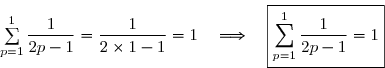
![F_2(x)=\displaystyle\int_{0}^{x}\Big(f_1^{-1}(t)\Big)^{2}\,\text{d}t \\\overset{ { \white{ . } } } {\phantom{F_2(x)}=\displaystyle\int_{0}^{x}\bigg(1-\Big((f_1)^{-1}(t)\Big)'\bigg)\,\text{d}t} \\\overset{ { \white{ . } } } {\phantom{F_2(x)}=\displaystyle\int_{0}^{x}1\,\text{d}t-\displaystyle\int_{0}^{x}\,\Big((f_1)^{-1}(t)\Big)'\bigg)\,\text{d}t} \\\overset{ { \white{ . } } } {\phantom{F_2(x)}=\bigg[t-(f_1)^{-1}(t)\bigg]_0^x}](https://latex.ilemaths.net/latex-0.tex?F_2(x)=\displaystyle\int_{0}^{x}\Big(f_1^{-1}(t)\Big)^{2}\,\text{d}t \\\overset{ { \white{ . } } } {\phantom{F_2(x)}=\displaystyle\int_{0}^{x}\bigg(1-\Big((f_1)^{-1}(t)\Big)'\bigg)\,\text{d}t} \\\overset{ { \white{ . } } } {\phantom{F_2(x)}=\displaystyle\int_{0}^{x}1\,\text{d}t-\displaystyle\int_{0}^{x}\,\Big((f_1)^{-1}(t)\Big)'\bigg)\,\text{d}t} \\\overset{ { \white{ . } } } {\phantom{F_2(x)}=\bigg[t-(f_1)^{-1}(t)\bigg]_0^x})
![\\\overset{ { \white{ . } } } {\phantom{F_2(x)}=[x-(f_1)^{-1}(x)]-[0-(f_1)^{-1}(0)]} \\\overset{ { \white{ . } } } {\phantom{F_2(x)}=x-(f_1)^{-1}(x)} \\\overset{ { \white{ . } } } {\phantom{F_2(x)}=x-1\times\Big (f_1^{-1}(x)\Big)^{2\times1-1}} \\\overset{ { \phantom{ . } } } {\phantom{F_2(x)}=x-\sum\limits_{p=1}^1\left(\dfrac{1}{2p-1}\right)\Big (f_1^{-1}(x)\Big)^{2p-1}} \\\\\Longrightarrow\quad\boxed{F_{2}(x)=x-\sum\limits_{p=1}^1\left(\dfrac{1}{2p-1}\right)\Big (f_1^{-1}(x)\Big)^{2p-1}}](https://latex.ilemaths.net/latex-0.tex?\\\overset{ { \white{ . } } } {\phantom{F_2(x)}=[x-(f_1)^{-1}(x)]-[0-(f_1)^{-1}(0)]} \\\overset{ { \white{ . } } } {\phantom{F_2(x)}=x-(f_1)^{-1}(x)} \\\overset{ { \white{ . } } } {\phantom{F_2(x)}=x-1\times\Big (f_1^{-1}(x)\Big)^{2\times1-1}} \\\overset{ { \phantom{ . } } } {\phantom{F_2(x)}=x-\sum\limits_{p=1}^1\left(\dfrac{1}{2p-1}\right)\Big (f_1^{-1}(x)\Big)^{2p-1}} \\\\\Longrightarrow\quad\boxed{F_{2}(x)=x-\sum\limits_{p=1}^1\left(\dfrac{1}{2p-1}\right)\Big (f_1^{-1}(x)\Big)^{2p-1}})
 alors elle est encore vraie au rang
 . })
=x-\sum\limits_{p=1}^n\left(\dfrac{1}{2p-1}\right)\Big (f_1^{-1}(x)\Big)^{2p-1}}) ,
, }(x)=x-\sum\limits_{p=1}^{n+1}\left(\dfrac{1}{2p-1}\right)\Big (f_1^{-1}(x)\Big)^{2p-1}})
![F_{2(n+1)}=F_{2n+2}=F_{2n}(x)-\dfrac{1}{2n+1}\Big (f_1^{-1}(x)\Big)^{2n+1}\quad(\text{voir question 2. a - Partie D}) \\\overset{ { \white{ . } } } { \phantom{F_{2(n+1)}=F_{2n+2}}=x-\sum\limits_{p=1}^n\left(\dfrac{1}{2p-1}\right)\Big (f_1^{-1}(x)\Big)^{2p-1}-\dfrac{1}{2n+1}\Big (f_1^{-1}(x)\Big)^{2n+1}} \\\overset{ { \white{ . } } } { \phantom{F_{2(n+1)}=F_{2n+2}}=x-\left[\sum\limits_{p=1}^n\left(\dfrac{1}{2p-1}\right)\Big (f_1^{-1}(x)\Big)^{2p-1}+\dfrac{1}{2(n+1)-1}\Big (f_1^{-1}(x)\Big)^{2(n+1)-1}\right]} \\\overset{ { \white{ . } } } { \phantom{F_{2(n+1)}=F_{2n+2}}=x-\sum\limits_{p=1}^{n+1}\left(\dfrac{1}{2p-1}\right)\Big (f_1^{-1}(x)\Big)^{2p-1}} \\\\\Longrightarrow\quad\boxed{F_{2(n+1)}=x-\sum\limits_{p=1}^{n+1}\left(\dfrac{1}{2p-1}\right)\Big (f_1^{-1}(x)\Big)^{2p-1}}](https://latex.ilemaths.net/latex-0.tex?F_{2(n+1)}=F_{2n+2}=F_{2n}(x)-\dfrac{1}{2n+1}\Big (f_1^{-1}(x)\Big)^{2n+1}\quad(\text{voir question 2. a - Partie D}) \\\overset{ { \white{ . } } } { \phantom{F_{2(n+1)}=F_{2n+2}}=x-\sum\limits_{p=1}^n\left(\dfrac{1}{2p-1}\right)\Big (f_1^{-1}(x)\Big)^{2p-1}-\dfrac{1}{2n+1}\Big (f_1^{-1}(x)\Big)^{2n+1}} \\\overset{ { \white{ . } } } { \phantom{F_{2(n+1)}=F_{2n+2}}=x-\left[\sum\limits_{p=1}^n\left(\dfrac{1}{2p-1}\right)\Big (f_1^{-1}(x)\Big)^{2p-1}+\dfrac{1}{2(n+1)-1}\Big (f_1^{-1}(x)\Big)^{2(n+1)-1}\right]} \\\overset{ { \white{ . } } } { \phantom{F_{2(n+1)}=F_{2n+2}}=x-\sum\limits_{p=1}^{n+1}\left(\dfrac{1}{2p-1}\right)\Big (f_1^{-1}(x)\Big)^{2p-1}} \\\\\Longrightarrow\quad\boxed{F_{2(n+1)}=x-\sum\limits_{p=1}^{n+1}\left(\dfrac{1}{2p-1}\right)\Big (f_1^{-1}(x)\Big)^{2p-1}} )
=x-\sum\limits_{p=1}^n\left(\dfrac{1}{2p-1}\right)\Big (f_1^{-1}(x)\Big)^{2p-1}}\,. })
-F_{2n}(f_1(x)).)
)=f_1(x)-\sum\limits_{p=1}^n\left(\dfrac{1}{2p-1}\right)\Big (f_1^{-1}(f_1(x))\Big)^{2p-1} \\\overset{ { \white{ . } } } { \quad\quad\Longleftrightarrow\quad F_{2n}(f_1(x))=f_1(x)-\sum\limits_{p=1}^n\left(\dfrac{1}{2p-1}\right)x^{2p-1}} \\\overset{ { \white{ . } } } { \quad\quad\Longleftrightarrow\quad \sum\limits_{p=1}^n\left(\dfrac{1}{2p-1}\right)x^{2p-1}=f_1(x)-F_{2n}(f_1(x))} \\\overset{ { \white{ . } } } { \quad\quad\Longleftrightarrow\quad \frac{1}{2-1}\,x+\frac{1}{4-1}\, x^3+\cdots+\dfrac{1}{2n-1}\,x^{2n-1}=f_1(x)-F_{2n}(f_1(x))} \\\overset{ { \phantom{ . } } } { \quad\quad\Longleftrightarrow\quad \boxed{x+\dfrac13 x^3+\cdots+\dfrac{1}{2n-1}\,x^{2n-1}=f_1(x)-F_{2n}(f_1(x))}})
\times 3^{2n-1}} \right). })
 nous obtenons ainsi :
  ^3+\cdots+\dfrac{1}{2n-1}\times\left(\dfrac13\right) ^{2n-1}=f_1\left(\frac13\right) -F_{2n}(f_1\left(\frac13\right) ) \\\overset{ { \white{ . } } } {\phantom{XXX}\Longleftrightarrow\quad \dfrac13+\dfrac{1}{3\times3^3}+\cdots+\dfrac{1}{(2n-1)\times3^{2n-1}}=f_1\left(\frac13\right) -F_{2n}(f_1\left(\frac13\right) )})
=\dfrac12\,\ln\left(\dfrac{1+\frac13}{1-\frac13}\right) \\\phantom{XXXXX}=\dfrac12\,\ln\left(\dfrac{\frac43}{\frac23}\right)\\\phantom{XXXXX}=\dfrac12\ln2\\\phantom{XXXXX}=\ln\sqrt2\\\\\Longrightarrow\quad f_1\left(\frac13\right)=\ln\sqrt2 \\\\\text{D'où }\;\lim\limits_{n\to+\infty}\left( \dfrac13+\dfrac{1}{3\times 3^3}+\cdots++\dfrac{1}{(2n-1)\times 3^{2n-1}} \right)=\ln\sqrt2-\lim\limits_{n\to+\infty}F_{2n}(\ln\sqrt2))
=0. })

=0. })
\times 3^{2n-1}} \right)=\ln\sqrt2-0\,, })
\times 3^{2n-1}} \right)=\ln\sqrt2}\,. }) Publié par malou
le
Publié par malou
le
 Voir la correction
 forum de terminale