1. Soit la fonction numérique à variable réelle définie par Quel est l'ensemble de définition de ? Réponse D :
En effet,
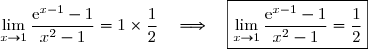
2.Quelle est la limite quand tend vers 1 de ? Réponse B :
En effet,
Par conséquent,
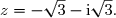
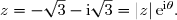
3.Quelle est l'écriture sous forme exponentielle du nombre complexe Réponse B :
En effet,
Déterminons le module de
Déterminons un argument de
Dès lors,
D'où, une écriture exponentielle de est
4.Soit définie par Quelle est l'expression de sa dérivée ?
Réponse D :
En effet,
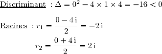
5.Quelle est l'expression de la solution de l'équation différentielle vérifiant et ?
Réponse C :
Première méthode : Vérification.
Soit
De plus
et
Par conséquent, l'expression de la solution de l'équation différentielle vérifiant et est
Deuxième méthode : Résolution détaillée.
À l'équation différentielle , nous associons l'équation caractéristique
Résolvons cette équation caractéristique.
Puisque l'équation caractéristique admet deux racines complexes conjuguées et , les solutions de l'équation différentielles s'écrivent sous la forme :
, soit
D'où les solutions de l'équation différentielles s'écrivent sous la forme :
De plus,
Par conséquent, l'expression de la solution de l'équation différentielle vérifiant et est
4 points
exercice 2
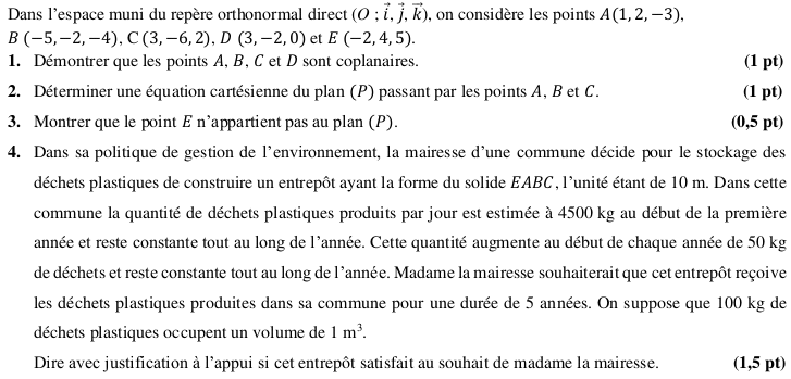
Dans l'espace muni du repère orthonormal direct on considère les points suivants :
et
1. Nous devons démontrer que les points A, B, C et D sont coplanaires.
Montrons que
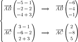
Déterminons les coordonnées du vecteur
Nous en déduisons que
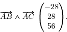
D'où nous obtenons le vecteur
Le vecteur n'est pas le vecteur nul.
Dès lors, les vecteurs et ne sont pas colinéaires.
Par conséquent, les points A, B et C déterminent un plan
De plus,
Par conséquent, les points A, B, C et D sont coplanaires.
2. Déterminons une équation cartésienne du plan passant par les points A, B et C .
Le vecteur est un vecteur normal au plan
D'où l'équation du plan est de la forme où est un nombre réel.
Nous savons que appartient à ce plan.
Donc soit
Par conséquent, une équation cartésienne du plan est
En divisant les deux membres de l'équation par (-28), nous obtenons :
3. Le point n'appartient pas au plan car ses coordonnées ne vérifient pas l'équation du plan.
En effet,
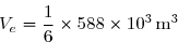
4. Soit le volume exprimé en m3 de l'entrepôt le volume total exprimé en m3 occupé par les déchets plastiques pour la durée de 5 ans.
Pour savoir si cet entrepôt satisfait au souhait de la mairesse, nous allons comparer et
Calculons le volume de l'entrepôt.
Le solide EABC est un tétraèdre car le point n'appartient pas au plan .
Si la base de ce tétraèdre est le triangle ABC , le volume de l'entrepôt se calcule par
En nous aidant des résultats de la question 1, nous obtenons :
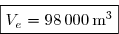
Dès lors, le volume de l'entrepôt est égal à , soit
Calculons le volume occupé par les déchets plastiques pour la durée de 5 ans.
Notons la quantité (exprimée en kg) de déchets plastiques produits dans la commune durant la nième année.
Lors de la première année, chaque jour, il est produit 4500 kg de déchets plastiques.
Donc la quantité (exprimée en kg) de déchets plastiques produits durant la première année est
Ensuite, au premier jour de chaque année, la quantité de déchets plastiques augmente de 50 kg et reste constante tout au long de l'année.
Nous en déduisons que pour tout entier naturel n non nul,
Par conséquent, est une suite arithmétique de raison dont le premier terme est
Dès lors, le terme général de la suite est , soit
En particulier, la quantité (exprimée en kg), de déchets plastiques produits dans la commune durant la 5ième année est , soit
La quantité de déchets plastiques produits pour une durée de 5 ans est la somme des 5 premiers termes de la suite
Cette somme se calcule par
Donc
Or 100 kg de déchets plastiques occupent un volume de 1 m3.
Dès lors, le volume occupé par les déchets plastiques est égal à , soit
Nous observons que
Nous pouvons donc affirmer que cet entrepôt satisfait au souhait de madame la mairesse.
11 points
probleme
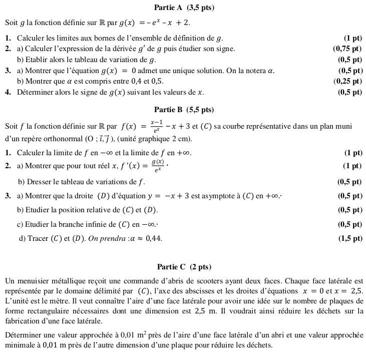
Partie A (3,5 points)
Soit la fonction définie sur par
1. Nous devons calculer les limites aux bornes de l'ensemble de définition de
L'ensemble de définition de est
Calculons
D'où
Calculons
D'où
2. a) Déterminons l'expression algébrique de et étudions son signe.
La fonction est dérivable sur et
Étudions le signe de
2. b) Étudions les variations de
Nous savons par la question précédente que
Nous en déduisons que la fonction est strictement décroissante sur
Dressons le tableau de variations de
3. a) Montrons que l'équation admet une solution unique (notée ).
La fonction g est continue et strictement décroissante sur
Il s'ensuit que g réalise une bijection de sur
Or
Dès lors, l'équation admet une unique solution sur
3. b)
D'où
4. Nous devons en déduire le signe de
Complétons le tableau de variations de
Nous en déduisons que sur sur
Partie B (5,5 points)
Soit la fonction définie sur par
1. Nous devons calculer la limite de en - et la limite de en +.
Calculons
D'où
Par conséquent,
Calculons
Par conséquent,
2. a) La fonction est dérivable sur
Pour tout
2. b) Étudions les variations de
Puisque l'exponentielle est toujours strictement positive, nous en déduisons que le signe de est le signe de
En nous basant sur le signe de étudié dans la partie A - question 5, nous en déduisons le tableau de variations de
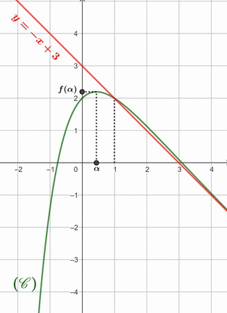
3. a) Nous devons montrer que la droite d'équation est asymptote à en +.
Il s'ensuit que la droite d'équation est asymptote à en +.
3. b) Étudions la position relative de et de
Étudions le signe de
Pour tout réel ,
Par conséquent, sur ]- ; 1[, la courbe est en dessous de la droite , sur ]1 ; +[, la courbe est au-dessus de la droite
3. c) Étudions la branche infinie de en -.
Donc la courbe admet une branche parabolique de direction l'axe des ordonnées en -.
3. d) Traçons et dans un repère orthonormal
Remarque :
Partie C (2 points)
Déterminons une valeur approchée à 0,01 m2 près de l'aire d'une face latérale d'un abri.
L'aire est donnée par :
Calculons
Nous obtenons ainsi :
soit
L'autre dimension de la plaque est donnée par le maximum de la fonction , soit
Par conséquent, la valeur approchée de l'autre dimension est 2,20 m (à 0,01 m près).
Publié par malou
le
ceci n'est qu'un extrait
Pour visualiser la totalité des cours vous devez vous inscrire / connecter (GRATUIT) Inscription Gratuitese connecter
Merci à Hiphigenie / malou pour avoir contribué à l'élaboration de cette fiche
Désolé, votre version d'Internet Explorer est plus que périmée ! Merci de le mettre à jour ou de télécharger Firefox ou Google Chrome pour utiliser le site. Votre ordinateur vous remerciera !
 la fonction numérique à variable réelle définie par
 =\ln(x^2). })
 Quel est l'ensemble de définition de

\in\R\quad\Longleftrightarrow\quad x^2>0 \\\phantom{\ln(x^2)\in\R}\quad\Longleftrightarrow\quad x\neq0 \\\phantom{\ln(x^2)\in\R}\quad\Longleftrightarrow\quad x\in\R\,\setminus\,\lbrace 0 \rbrace)

 tend vers 1 de
  ?
?
(x+1)} \\\overset{ { \white{ . } } } {\phantom{\lim\limits_{x\to1}\dfrac{\text e^{x-1}-1}{x^2-1}}=\lim\limits_{x\to1}\left(\dfrac{\text e^{x-1}-1}{x-1}\times\dfrac{1}{x+1}\right)} \\\overset{ { \white{ . } } } {\phantom{\lim\limits_{x\to1}\dfrac{\text e^{x-1}-1}{x^2-1}}=\lim\limits_{x\to1}\dfrac{\text e^{x-1}-1}{x-1}\times\lim\limits_{x\to1}\dfrac{1}{x+1}})
\quad\text{où }f\text{ est définie sur }\R\text{ par }f(t)=\text e^t} \\\overset{ { \white{ . } } } {\phantom{\text{Or }\;\lim\limits_{x\to1}\dfrac{\text e^{x-1}-1}{x-1}}=1\quad\text{(car }f'(t)=\text e^t\Longrightarrow f'(0)=\text e^0=1)} \\\\\text{et }\;\lim\limits_{x\to1}\dfrac{1}{x+1}=\dfrac{1}{1+1}=\dfrac12)


 Déterminons le module de
^2+(-\sqrt3)^2}=\sqrt{3+3}=\sqrt6\quad\Longrightarrow\quad \boxed{|z|=\sqrt 6})
 de
de  \\\\\overset{ { \white{ . } } } {\quad\Longrightarrow\quad\sqrt6\,(\cos\theta+\text i\sin\theta)=-\sqrt3-\text i\sqrt3} \\\overset{ { \white{ . } } } {\quad\Longrightarrow\quad \cos\theta+\text i\sin\theta=-\dfrac{\sqrt3}{\sqrt6}-\text i\dfrac{\sqrt3}{\sqrt6}} \\\overset{ { \white{ . } } } {\quad\Longrightarrow\quad \cos\theta+\text i\sin\theta=-\dfrac{1}{\sqrt2}-\text i\dfrac{1}{\sqrt2}} \\\overset{ { \white{ . } } } {\quad\Longrightarrow\quad \cos\theta+\text i\sin\theta=-\dfrac{\sqrt2}{2}-\text i\dfrac{\sqrt2}{2}})
![\left\lbrace\begin{matrix}\cos\theta=-\dfrac{\sqrt2}{2}\\\overset{ { \white{ . } } } {\sin\theta=-\dfrac{\sqrt2}{2}}\end{matrix}\right.\quad\Longrightarrow\quad\theta=-\dfrac{3\pi}{4}\,[2\pi],\text{ ou encore }\boxed{\theta=\dfrac{5\pi}{4}\,[2\pi]}](https://latex.ilemaths.net/latex-0.tex?\left\lbrace\begin{matrix}\cos\theta=-\dfrac{\sqrt2}{2}\\\overset{ { \white{ . } } } {\sin\theta=-\dfrac{\sqrt2}{2}}\end{matrix}\right.\quad\Longrightarrow\quad\theta=-\dfrac{3\pi}{4}\,[2\pi],\text{ ou encore }\boxed{\theta=\dfrac{5\pi}{4}\,[2\pi]})
 est
est 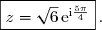
 définie par
 =x^3\,(\ln x)^2. })
.}} })
=\Big(x^3\,(\ln x)^2\Big)' \\\overset{ { \white{ . } } } {\phantom{f'(x)}=(x^3)'\times\,(\ln x)^2+x^3\times\,\Big((\ln x)^2\Big)'} \\\overset{ { \white{ . } } } {\phantom{f'(x)}=3x^2\times\,(\ln x)^2+x^3\times\,2\times\dfrac1x\times\ln x} \\\overset{ { \white{ . } } } {\phantom{f'(x)}=3x^2(\ln x)^2+2x^2\ln x} \\\overset{ { \phantom{ . } } } {\phantom{f'(x)}=x^2\ln x(3\ln x+2)} \\\\\Longrightarrow\quad\boxed{f'(x)=x^2\ln x(3\ln x+2)})
 vérifiant
 =1 }) et
et =0 }) ?
?
=\cos 2x. })
=\cos 2x\quad\Longrightarrow\quad y'(x)=-2\sin 2x \\\overset{ { \white{ . } } } {\phantom{y(x)=\cos 2x}\quad\Longrightarrow\quad y''(x)=-4\cos 2x} \\\\\text{D'où }\;y''(x)+4y(x)=-4\cos 2x+4\cos2x=0\quad\Longrightarrow\quad \boxed{y''(x)+4y(x)=0})
=\cos0\quad\Longrightarrow\quad \boxed{y(0)=1}})
=-2\sin 0\quad\Longrightarrow\quad \boxed{y'(0)=0}})
 vérifiant
 =\cos 2x}\,. })


 et
et  , les solutions de l'équation différentielles s'écrivent sous la forme :
=\text e^{0 x}(\alpha\cos 2x+\beta\sin 2x)}) , soit
, soit =\alpha\cos 2x+\beta\sin 2x\quad\quad(\alpha\in\R\,,\beta\in\R)}})
=1\quad\Longrightarrow\quad \alpha\cos 0+\beta\sin 0=1 \\\phantom{\text{Or }\;y(0)=1}\quad\Longrightarrow\quad \alpha\times1+\beta\times0=1 \\\phantom{\text{Or }\;y(0)=1}\quad\Longrightarrow\quad \boxed{\alpha=1})
=\cos 2x+\beta\sin 2x\quad\quad(\beta\in\R)}})
=\cos 2x+\beta\sin 2x\quad\Longrightarrow\quad y'(x)=-2\sin 2x+2\beta\cos 2x. })
=0\quad\Longrightarrow\quad -2\sin 0+2\beta\cos 0=0 \\\phantom{\text{Dès lors, }\;y'(0)=0}\quad\Longrightarrow\quad 2\beta=0 \\\phantom{\text{Dès lors, }\;y'(0)=0}\quad\Longrightarrow\quad \beta=0)
, }) on considère les points suivants :
on considère les points suivants : ,\,B(-5\;;\;-2\;;\;-4),\,C(3\;;\;-6\;;\;2)},\,D(3\;;\;-2\;;\;0)) et
et .})
\cdot\overrightarrow{AD}=0.})

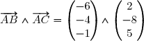

\times5-(-1)\times(-8)\\ (-1)\times2-(-6)\times5\\ (-6)\times(-8)-(-4)\times2\end{pmatrix}} \\\overset{ { \white{ . } } } {\phantom{WWWWWWWW}=\begin{pmatrix}-28\\28\\56\end{pmatrix}})
 n'est pas le vecteur nul.
 et
et  ne sont pas colinéaires.
. })
\cdot\overrightarrow{AD}=(-28)\times2+28\times(-4)+56\times3} \\\phantom{WWWWWwWWW}\quad\Longrightarrow\quad \boxed{\left(\overrightarrow{AB}\wedge\overrightarrow{AC}\right)\cdot\overrightarrow{AD}=0})
 }) passant par les points A, B et C .
passant par les points A, B et C .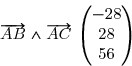 est un vecteur normal au plan
 . })
}) est de la forme
est de la forme 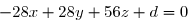 où
où  est un nombre réel.
 }) appartient à ce plan.
appartient à ce plan.+d=0, }) soit
soit 
 }) est
est 
 : x-y-2z-5=0}\,. })
}) n'appartient pas au plan
n'appartient pas au plan 
 le volume exprimé en m3 de l'entrepôt
 le volume total exprimé en m3 occupé par les déchets plastiques pour la durée de 5 ans.
 n'appartient pas au plan
 \cdot\overrightarrow{AE}\right|\times 10^3\,\text{m}^3. })
\cdot\overrightarrow{AE}=(-28)\times(-3)+28\times2+56\times8} \\\phantom{WWWWWwWWW}\quad\Longrightarrow\quad \boxed{\left(\overrightarrow{AB}\wedge\overrightarrow{AC}\right)\cdot\overrightarrow{AE}=588})
 ,
, 
 la quantité (exprimée en kg) de déchets plastiques produits dans la commune durant la n ième année.

 }) est une suite arithmétique de raison
est une suite arithmétique de raison  dont le premier terme est
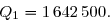
\times r }) ,
, \times 18\,250}\,. })
 , soit
. })

 ,
, 

 la fonction définie sur
  par
par =-\,\text e^x-x+2. })


. })
=+\infty)
=+\infty}\,. })
. })
=-\infty)
=-\infty}\,. })
 }) et étudions son signe.
et étudions son signe. est dérivable sur
  et
et =-\text e^x-1})
. })
<0 \\\\\Longrightarrow\boxed{\forall\,x\in\,\R,\;g'(x)<0}\,.)

<0. } )
&&-&-&-&-&-&\\&&&&&&&\\\hline&+\infty&&&&&&\\g(x)&||&\searrow&\searrow&\searrow&\searrow&\searrow&\\&||&&&&&&-\infty\\\hline \end{array} )
=0 }) admet une solution unique (notée
admet une solution unique (notée  ).
). sur
sur ![\overset{ { \white{ . } } } { g( \R)=\,]-\infty\;;\;+\infty[\,=\R.}](https://latex.ilemaths.net/latex-0.tex?\overset{ { \white{ . } } } { g( \R)=\,]-\infty\;;\;+\infty[\,=\R.})

=0}) admet une unique solution
admet une unique solution  sur
sur 
\approx0,108>0\phantom{x}\\\overset{ { \white{ . } } } {g(0,5)\approx-0,149<0}\end{matrix}\right.\quad\Longrightarrow\quad g(0,4)\times g(0,5)<0)
 D'où
D'où 


&||&\searrow&\searrow&0&\searrow&\searrow&\\&||&&&&&&-\infty\\\hline \end{array} )
>0 }) sur
sur ![\overset{ { \white{ . } } } { ]-\infty\;;\;\alpha\,[ }](https://latex.ilemaths.net/latex-0.tex?\overset{ { \white{ . } } } { ]-\infty\;;\;\alpha\,[ })

<0 }) sur
sur ![\overset{ { \white{ . } } } { ]\,\alpha\;;\;+\infty\,[. }](https://latex.ilemaths.net/latex-0.tex?\overset{ { \white{ . } } } { ]\,\alpha\;;\;+\infty\,[. })
 la fonction définie sur
 =\dfrac{x-1}{\text e^x}-x+3. })
 et la limite de
 . })
=\lim\limits_{x\to-\infty}\left(\dfrac{x-1}{\text e^x}-x+3\right)=\lim\limits_{x\to-\infty}\left(\dfrac{x-1-x\,\text e^x+3\,\text e^x}{\text e^x}\right) \\\\\text{Or }\left\lbrace\begin{matrix}\lim\limits_{x\to-\infty}(x-1)=-\infty\phantom{WWWWWWWW}\\\lim\limits_{x\to-\infty}x\,\text e^x=0\quad(\text{croissances comparées)}\\\lim\limits_{x\to-\infty}3\,\text e^x=0\phantom{WWWWWWWWWWw}\end{matrix}\right.\\\\\quad\Longrightarrow\quad\lim\limits_{x\to-\infty}(x-1-x\,\text e^x+3\,\text e^x)=-\infty)
=-\infty \\\lim\limits_{x\to-\infty}\text e^x=0^+\phantom{WWWWWWWW}\end{matrix}\right.\quad\Longrightarrow\quad\lim\limits_{x\to-\infty}\left(\dfrac{x-1-x\,\text e^x+3\,\text e^x}{\text e^x}\right)=-\infty})
=-\infty}\,. })
. })
=\lim\limits_{x\to+\infty}\left(\dfrac{x-1}{\text e^x}-x+3\right) \\\\\text{Or }\lim\limits_{x\to+\infty}\dfrac{x-1}{\text e^x}=0\quad(\text{croissances comparées)}\\\\\quad\Longrightarrow\quad\lim\limits_{x\to+\infty}\left(\dfrac{x-1}{\text e^x}-x+3\right)=-\infty)
=-\infty}\,. })


=\left(\dfrac{x-1}{\text e^x}-x+3\right)' \\\overset{ { \white{ . } } } {\phantom{f(x)}=\left(\dfrac{x-1}{\text e^x}\right)'-1} \\\overset{ { \white{ . } } } {\phantom{f(x)}=\dfrac{(x-1)'\times\text e^x-(x-1)\times (\text e^x)'}{(\text e^x)^2}-1} \\\overset{ { \white{ . } } } {\phantom{f(x)}=\dfrac{1\times\text e^x-(x-1)\times \text e^x}{\text e^{2x}}-1})
}=\dfrac{\text e^x-(x-1)\times \text e^x}{\text e^{2x}}-1} \\\overset{ { \white{ . } } } {\phantom{f(x)}=\dfrac{\text e^x(1-x+1)}{\text e^{2x}}-1} \\\overset{ { \white{ . } } } {\phantom{f(x)}=\dfrac{\text 2-x}{\text e^{x}}-1} \\\overset{ { \phantom{ . } } } {\phantom{f(x)}=\dfrac{\text 2-x-\text e^{x}}{\text e^{x}}} \\\overset{ { \phantom{ . } } } {\phantom{f(x)}=\dfrac{g(x)}{\text e^{x}}} \\\\\Longrightarrow\quad\boxed{\forall\,x\in\R,\;f'(x)=\dfrac{g(x)}{\text e^{x}}} )

 } ) est le signe de
est le signe de  .} )
&&+&+&0&-&-&\\&&&&&&&\\\hline&&&&f(\alpha)&&&\\f(x)&&\nearrow&\nearrow&&\searrow&\searrow&\\&-\infty&&&&&&-\infty\\\hline \end{array} )
 }) d'équation
d'équation  est asymptote à
  }) en +
en +-(-x+3)}\right)=\lim\limits_{x\to+\infty}\dfrac{x-1}{\text e^x}=0\quad(\text{croissances comparées}) \\\\\Longrightarrow\quad\boxed{\lim\limits_{x\to+\infty}\left(\overset{}{f(x)-(-x+3)}\right)=0})
. })
-(-x+3). })
-(-x+3)=\dfrac{x-1}{\text e^x}. })

 }) ,
, sur ]1 ; +
}{x}=\lim\limits_{x\to -\infty}\left(\dfrac{x-1}{x\,\text e^x}-\dfrac{x}{x}+\dfrac3x\right) \\\overset{ { \white{ . } } } { \phantom{\lim\limits_{x\to -\infty}\dfrac{f(x)}{x}}=\lim\limits_{x\to -\infty}\left(\dfrac{x-1}{x\,\text e^x}-1+\dfrac3x\right)})
 \\\overset{ { \white{ . } } } { \phantom{\text{Or }\;\lim\limits_{x\to -\infty}\dfrac{x-1}{x\,\text e^x}}=\lim\limits_{x\to -\infty}\dfrac{x-1}{x}\times\lim\limits_{x\to -\infty}\dfrac{1}{\text e^x}} \\\overset{ { \white{ . } } } { \phantom{\text{Or }\;\lim\limits_{x\to -\infty}\dfrac{x-1}{x\,\text e^x}}=\lim\limits_{x\to -\infty}\dfrac{x}{x}\times\lim\limits_{x\to -\infty}\dfrac{1}{\text e^x}} \\\overset{ { \phantom{ . } } } { \phantom{\text{Or }\;\lim\limits_{x\to -\infty}\dfrac{x-1}{x\,\text e^x}}=1\times(+\infty)=+\infty})
}{x}=\lim\limits_{x\to -\infty}\left(\dfrac{x-1}{x\,\text e^x}-1+\dfrac3x\right)=+\infty-1+0=+\infty \\\\\Longrightarrow\quad\boxed{\lim\limits_{x\to -\infty}\dfrac{f(x)}{x}=+\infty})
. })

\approx2,2. })
 d'une face latérale d'un abri.
\,\text{d}x. })
\,\text{d}x \\\overset{ { \white{ . } } } { \phantom{A}=\displaystyle\int_{0}^{2,5} \Big(\dfrac{x-1}{\text e^x}-x+3\Big) \,\text{d}x} \\\overset{ { \white{ . } } } { \phantom{A}=\displaystyle\int_{0}^{2,5} (x-1)\,\text e^{-x} \,\text{d}x+\displaystyle\int_{0}^{2,5}(- x +3)\,\text{d}x} )
 \,\text{d}x} \\\overset{ { \white{ . } } } { \phantom{A}=\displaystyle\int_{0}^{2,5} x\,\text e^{-x}\,\text{d}x+\displaystyle\int_{0}^{2,5} -\text e^{-x}\,\text{d}x+\displaystyle\int_{0}^{2,5}(-x+3) \,\text{d}x})
![\\\overset{ { \white{ . } } } { \phantom{A}=\displaystyle\int_{0}^{2,5} x\,\text e^{-x}\,\text{d}x+\left[\overset{}{\text e^{-x}}\right]_0^{2,5}+\left[\overset{}{-\dfrac{x^2}{2}}+3x\right]_0^{2,5}} \\\overset{ { \white{ . } } } { \phantom{A}=\displaystyle\int_{0}^{2,5} x\,\text e^{-x}\,\text{d}x+(\text e^{-2,5}+\text e^0)+\left(-\dfrac{2,5^2}{2}+3\times2,5\right)-0} \\\overset{ { \white{ . } } } { \phantom{A}=\displaystyle\int_{0}^{2,5} x\,\text e^{-x}\,\text{d}x+\text e^{-2,5}-1-\dfrac{6,25}{2}+7,5} \\\overset{ { \phantom{ . } } } { \phantom{A}=\displaystyle\int_{0}^{2,5} x\,\text e^{-x}\,\text{d}x+\text e^{-2,5}+3,375}](https://latex.ilemaths.net/latex-0.tex?\\\overset{ { \white{ . } } } { \phantom{A}=\displaystyle\int_{0}^{2,5} x\,\text e^{-x}\,\text{d}x+\left[\overset{}{\text e^{-x}}\right]_0^{2,5}+\left[\overset{}{-\dfrac{x^2}{2}}+3x\right]_0^{2,5}} \\\overset{ { \white{ . } } } { \phantom{A}=\displaystyle\int_{0}^{2,5} x\,\text e^{-x}\,\text{d}x+(\text e^{-2,5}+\text e^0)+\left(-\dfrac{2,5^2}{2}+3\times2,5\right)-0} \\\overset{ { \white{ . } } } { \phantom{A}=\displaystyle\int_{0}^{2,5} x\,\text e^{-x}\,\text{d}x+\text e^{-2,5}-1-\dfrac{6,25}{2}+7,5} \\\overset{ { \phantom{ . } } } { \phantom{A}=\displaystyle\int_{0}^{2,5} x\,\text e^{-x}\,\text{d}x+\text e^{-2,5}+3,375})

![\underline{\text{Formule de l'intégrale par parties}}\ :\ {\blue{\displaystyle\int_0^{2,5}u(x)v'(x)\,\text{d}x=\left[\overset{}{u(x)v(x)}\right]\limits_0^{2,5}- \displaystyle\int\limits_0^{2,5}u'(x)v(x)\,\text{d}x}}. \\ \\ \left\lbrace\begin{matrix}u(x)=x\quad\Longrightarrow\quad u'(x)=1 \\\\v'(x)=\text e^{-x}\phantom{}\quad\Longrightarrow\quad v(x)=-\text e^{-x}\end{matrix}\right.](https://latex.ilemaths.net/latex-0.tex?\underline{\text{Formule de l'intégrale par parties}}\ :\ {\blue{\displaystyle\int_0^{2,5}u(x)v'(x)\,\text{d}x=\left[\overset{}{u(x)v(x)}\right]\limits_0^{2,5}- \displaystyle\int\limits_0^{2,5}u'(x)v(x)\,\text{d}x}}. \\ \\ \left\lbrace\begin{matrix}u(x)=x\quad\Longrightarrow\quad u'(x)=1 \\\\v'(x)=\text e^{-x}\phantom{}\quad\Longrightarrow\quad v(x)=-\text e^{-x}\end{matrix}\right.)
![\text{Dès lors }\;\overset{ { \white{ . } } } { \displaystyle\int_{0}^{2,5} x\,\text e^{-x}\,\text{d}x=\left[\overset{}{-x\,\text e^{-x}}\right]_0^{2,5}-\displaystyle\int_0^{2,5}1\times(-\text{e}^{-x})\,\text{d}x} \\\overset{ { \white{ . } } } {\phantom{WWWWWWWWW}=\left[\overset{}{-x\,\text e^{-x}}\right]_0^{2,5}-\displaystyle\int_0^{2,5}-\text{e}^{-x}\,\text{d}x} \\\overset{ { \phantom{ . } } } {\phantom{WWWWWWWWW}=\left[\overset{}{-x\,\text e^{-x}}\right]_0^{2,5}-\left[\overset{}{\text e^{-x}}\right]_0^{2,5}} \\\overset{ { \phantom{ . } } } {\phantom{WWWWWWWWW}=(-2,5\,\text e^{-2,5}-0)-(\text e^{-2,5}-\text e^0)} \\\overset{ { \white{ . } } } {\phantom{WWWWWWWWW}=-2,5\,\text e^{-2,5}-\text e^{-2,5}+1} \\\overset{ { \phantom{ . } } } { \phantom{WWWWWWWWW}=-3,5\,\text e^{-2,5}+1}](https://latex.ilemaths.net/latex-0.tex?\text{Dès lors }\;\overset{ { \white{ . } } } { \displaystyle\int_{0}^{2,5} x\,\text e^{-x}\,\text{d}x=\left[\overset{}{-x\,\text e^{-x}}\right]_0^{2,5}-\displaystyle\int_0^{2,5}1\times(-\text{e}^{-x})\,\text{d}x} \\\overset{ { \white{ . } } } {\phantom{WWWWWWWWW}=\left[\overset{}{-x\,\text e^{-x}}\right]_0^{2,5}-\displaystyle\int_0^{2,5}-\text{e}^{-x}\,\text{d}x} \\\overset{ { \phantom{ . } } } {\phantom{WWWWWWWWW}=\left[\overset{}{-x\,\text e^{-x}}\right]_0^{2,5}-\left[\overset{}{\text e^{-x}}\right]_0^{2,5}} \\\overset{ { \phantom{ . } } } {\phantom{WWWWWWWWW}=(-2,5\,\text e^{-2,5}-0)-(\text e^{-2,5}-\text e^0)} \\\overset{ { \white{ . } } } {\phantom{WWWWWWWWW}=-2,5\,\text e^{-2,5}-\text e^{-2,5}+1} \\\overset{ { \phantom{ . } } } { \phantom{WWWWWWWWW}=-3,5\,\text e^{-2,5}+1})
+\text e^{-2,5}+3,375)
\;\text{m}^2\approx4,17\;\text{m}^2})
\approx2,20 .})
 Voir la correction
 forum de terminale