Le plan est rapporté à un repère orthonormal direct
Soit l'ensemble et f l'application telle que :
1. Nous devons résoudre dans , l'équation
D'où, l'ensemble des solutions de l'équation est
2. a)
2. b) Soit tel que et
Par la question précédente nous savons que
Or,
Dès lors,
3. Nous devons déterminer l'ensemble des points M d'affixe z tels que : et f (z ) soit un réel.
Soit
Par conséquent, l'ensemble des points M d'affixe z tels que : et f (z ) soit un réel est la réunion de l'axe des abscisses et du cercle de rayon 1 centré en l'origine O du repère, privé des points J(0 ; 1) et J'(0 ; -1).
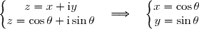
4. Dans cette question,
4. a) Nous devons montrer que f (z ) est réel et le calculer en fonction de cos.
L'ensemble des points d'affixe z tels que est le cercle de rayon 1 centré en l'origine O du repère, privé des points J(0 ; 1) et J'(0 ; -1).
Or nous avons montré dans la question 3 que ces points étaient tels que et f (z ) soit un réel.
Par conséquent, f (z ) est un réel.
Nous savons que
Dès lors,
En utilisant les résultats de la question 3. et en sachant que f (z ) est un réel, nous en déduisons que :
4. b) Soit la suite réelle telle que :
un est la somme de (n + 1) termes d'une suite géométrique de raison f (z ) dont le premier terme est 1.
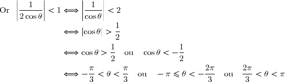
La suite convergera si la suite converge, soit si
Par conséquent, la suite (un ) converge si
4 points
exercice 2
Soit a un réel strictement positif.
Soit ABC un triangle équilatéral direct de côté de longueur a .
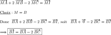
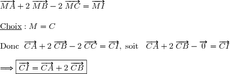
On note I le barycentre des points (A ; 1), (B ; 2) et (C ; -2).
1. Le point I est le barycentre des points (A ; 1), (B ; 2) et (C ; -2).
Donc pour tout point M du plan, nous obtenons :
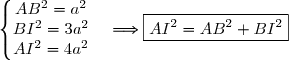
2.Calculons IA2.
Calculons IB2.
Pour tout point M du plan, nous savons que :
Calculons IC2.
Pour tout point M du plan, nous savons que :
3. Soit k un nombre réel.
3. a) Nous devons déterminer en fonction de k l'ensemble (k) des points M du plan tels que :
Par conséquent,
si k > -4, l'ensemble (k) est le cercle de centre I de rayon si k = -4, alors M = I et par suite, si k < -4, l'ensemble (k) est l'ensemble vide.
3. b)
Or nous avons montré dans la question 2. que
D'où,
Par conséquent, si k = -1.
4. a) Nous devons démontrer que (-1) est un cercle tangent à la droite (AB ).
Nous savons que (k) est le cercle de centre I de rayon
Donc (-1) est le cercle de centre I de rayon
Nous avons démontré dans la question 3. b) que si k = -1, soit que
Nous obtenons alors les résultats suivants :
Dès lors,
Par la réciproque du théorème de Pythagore, nous en déduisons que le triangle ABI est rectangle en B .
Il s'ensuit que la droite (AB ) est perpendiculaire au rayon en son extrémité sur le cercle (-1).
Par conséquent, la droite (AB ) est tangente au cercle (-1) au point B .
4. b) Nous devons montrer que le symétrique D du point B par rapport à la droite (AI ) appartient à la droite (AC ).
Soient les points M et N tels que et (voir figure à la question 1)
Par construction du point I , le quadrilatère AMIN est un losange car AM = MI = IN = AN = 2a .
D'où les diagonales [AI ] et [MN ] se coupent perpendiculairement en leurs milieux.
Nous en déduisons que le point N est le symétrique du point M par rapport à la droite (AI).
Puisque B appartient à la droite (AM), il en découle que le point D, symétrique du point B par rapport à la droite (AI ), appartient à la droite (AN ), soit à la droite (AC ).
Par conséquent, le point D appartient à la droite (AC ).
4. c) Nous devons démontrer que (-1) est tangent à la droite (AC ) en D .
Nous avons montré dans la question 4. a) que le triangle ABI est rectangle en B .
Or le triangle ADI est le symétrique du triangle ABI par rapport à la droite (AI )
Dès lors le triangle ADI est rectangle en D .
Il s'ensuit que (AD ) est perpendiculaire au rayon en son extrémité sur le cercle (-1).
D'où, la droite (AD ) est tangente au cercle (-1) au point D .
Puisque D appartient à la droite (AC ), les droites (AC ) et (AD ) sont confondues.
Par conséquent, la droite (AC ) est tangente au cercle (-1) au point D .
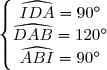
4. d) Nous devons déterminer la nature du triangle BID .
Montrons que le triangle BID est équilatéral.
Le triangle BID est isocèle en I car BI = ID = rayon du cercle (-1).
De plus, les points D , A et C sont alignés dans cet ordre.
.
Dans le quadrilatère DABI , nous savons que
Or
Nous obtenons alors :
En conclusion, le triangle BID est isocèle en I et l'angle du sommet principal I a une mesure de 60°.
Nous en déduisons que le triangle BID est équilatéral.
12 points
probleme
Soit la fonction et (Ca ) sa courbe représentative dans un plan rapporté à un repère orthonormal
Partie A :
1. Nous devons déterminer l'ensemble de définition Da de fa suivant les valeurs de a .
Envisageons deux cas.
Premier cas : a > 0.
La fonction fa est définie si
Or et nous savons que a > 0.
Donc
Par conséquent,
Deuxième cas : a 0.
La fonction fa est définie si
Par conséquent,
2. Nous devons étudier la dérivabilité de fa en 0 pour a > 0.
Premier cas : Étudions la dérivabilité de fa à droite de 0.
Nous savons que si x > 0, alors |x | = x .
Dès lors,
Posons
De plus, si alors
D'où,
Soit la fonction g définie sur par
Dans ce cas, représente la dérivée à droite de la fonction g en ln(a ).
Par conséquent,
Nous en déduisons que fa est dérivable à droite de 0 et que le nombre dérivé de fa à droite de 0 est égal à
Deuxième cas : Étudions la dérivabilité de fa à gauche de 0.
Nous savons que si x < 0, alors |x | = -x .
Dès lors,
Posons
De plus, si alors
D'où,
Soit la fonction g définie sur par
Dans ce cas, représente la dérivée à gauche de la fonction g en ln(a ).
Par conséquent,
Nous en déduisons que fa est dérivable à gauche de 0 et que le nombre dérivé de fa à gauche de 0 est égal à
Donc la fonction fa n'est pas dérivable en 0 car la dérivée à gauche de 0 est différente de la dérivée à droite de 0.
3. Etudions le sens de variation de fa suivant les valeurs de a .
Premier cas : a > 0.
Nous avons montré que et que la fonction fa n'est pas dérivable en 0.
Si x > 0, alors |x |=x et
Dans ce cas, , soit
Si x < 0, alors |x |=-x et
Dans ce cas, , soit
Par conséquent, si a > 0, alors la fonction fa est strictement croissante sur ]0 ; +[ et est strictement décroissante sur ]- ; 0[.
Deuxième cas : a 0.
Dans ce cas, -a 0 et nous avons montré que
Si x ]-a ; +[, alors x > 0 et par suite, |x |=x et
Nous obtenons alors, , soit
Si x ]- ; a[, alors x < 0 et par suite, |x | = -x et
Nous obtenons alors, , soit
Par conséquent, si a < 0, alors la fonction fa est strictement croissante sur ]-a ; +[ et est strictement décroissante sur ]- ; a [.
Dressons les tableaux de variation de fa suivant les valeurs de a . Calculs préliminaires :
D'où
4. a) Soit M (x ; y ) un point du plan.
Par conséquent, si , alors pour tout a'a ,
De même,
4. c) Nous en déduisons que les courbes (Ca ) et (Ca' ) sont asymptotes.
5. Représentations graphiques de et
Partie B :
1.
D'où,
2. a) Nous devons montrer que sur ]0 ; +[, l'équation admet une unique solution .
Soit la fonction h définie sur ]0 ; +[ par
La fonction h est dérivable sur ]0 ; +[ (différence de deux fonctions dérivables sur ]0 ; +[).
Dès lors, la fonction h est strictement décroissante sur ]0 ; +[.
Dressons le tableau de variations de la fonction h sur ]0 ; +[.
Donc nous savons que : la fonction h est continue sur ]0 ; +[ (car dérivable sur ]0 ; +[), la fonction h est strictement décroissante sur ]0 ; +[.
De plus h (]0 ; +[) = ]- ; ln2[.
D'après le théorème de la bijection, la fonction h réalise une bijection de ]0 ; +[ dans ]- ; ln2[.
Or 0 ]- ; ln2[.
Nous en déduisons que l'équation admet une unique solution dans ]0 ; +[.
Par conséquent, sur ]0 ; +[, l'équation admet une unique solution .
2. b) La calculatrice n'étant pas autorisée, nous remarquons que :
Nous obtenons ainsi :
Or d'après le théorème de la bijection, la fonction réciproque est strictement décroissante sur ]- ; ln2[.
En appliquant h-1 à l'inégalité précédente, nous obtenons :
Par conséquent,
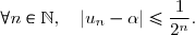
3. Soit la suite numérique définie par et pour tout entier naturel n ,
3. a) Montrons par récurrence que
Initialisation : Montrons que la propriété est vraie pour n = 0, soit que
La relation est évidente puisque et par conséquent, l'initialisation est vraie.
Hérédité : Montrons que si pour un nombre naturel n fixé, la propriété est vraie au rang n , alors elle est encore vraie au rang (n +1).
Montrons donc que si pour un nombre naturel n fixé, , alors
En effet,
Donc l'hérédité est vraie.
Puisque l'initialisation et l'hérédité sont vraies, nous avons montré par récurrence que
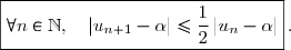
3. b) Nous devons montrer que
Soit et
La fonction f2 est continue sur l'intervalle [a ; b]. La fonction f2 est dérivable sur l'intervalle ]a ; b[. Nous savons que pour tout x ]0 ; +[, (voir question 1).
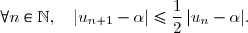
Selon l'inégalité des accroissements finis, nous savons que
Or et car est la solution de l'équation
Par conséquent,
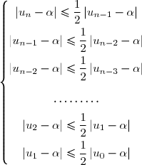
Montrons que L'inégalité est vraie si un = car elle s'écrirait : , ce qui est vrai par évidence.
Soit un.
Nous savons que
Dès lors, nous obtenons :
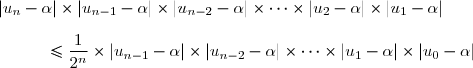
Multiplions ces n inégalités membre à membre.
Simplifions les facteurs identiques dans les deux membres.
Nous obtenons alors :
Or u0 = 1 et 1 2.
Nous déduisons alors que :
Il s'ensuit :
D'où
3. c) Déterminons à partir de quelle valeur n0 de n , un est une valeur approchée à 10-3 près de .
Nous savons que
Calculons la plus petite valeur entière naturelle de n vérifiant l'inéquation
Les valeurs suivantes sont données en fin de questionnaire :
Dès lors, la plus petite valeur entière naturelle de n vérifiant l'inéquation est n = 10.
Par conséquent, un est une valeur approchée à 10-3 près de à partir de n0 = 10.
Partie C :
On suppose que a > 1.
Soit H la partie du plan délimitée par (Ca ), (D ) : y = x + a et les droites d'équations x = 0 et x = a .
On note A (a ) l'aire de H .
1. Nous devons calculer A (a ) en fonction de a .
Sur l'intervalle [0 ; a ], l'expression de f (x ) est f (x ) = ln(x + a) car |x | = x puisque x 0.
Etudions la position relative de la droite (D) et de la courbe (Ca ) sur l'intervalle [0 ; a ].
Soit la fonction définie sur ]-a ; a ] par
La fonction est dérivable sur ]-a ; a ].
Nous en déduisons que sur l'intervalle [0 ; a ], (x ) > 1.
D'où, sur l'intervalle [0 ; a ], (x ) > 0, soit x + a > ln(x + a ).
Par conséquent, sur l'intervalle [0 ; a ], la droite (D) est située au-dessus de la courbe (Ca ).
Dès lors, A (a ) se détermine par :
Par conséquent,
Publié par malou
le
ceci n'est qu'un extrait
Pour visualiser la totalité des cours vous devez vous inscrire / connecter (GRATUIT) Inscription Gratuitese connecter
Merci à Hiphigenie / malou pour avoir contribué à l'élaboration de cette fiche
Désolé, votre version d'Internet Explorer est plus que périmée ! Merci de le mettre à jour ou de télécharger Firefox ou Google Chrome pour utiliser le site. Votre ordinateur vous remerciera !


.})
 l'ensemble
  et f l'application telle que :
 =\dfrac{z}{z^2+1}.})
=\dfrac{\sqrt{3}}{3}.)
=\dfrac{\sqrt{3}}{3}\Longleftrightarrow \dfrac{z}{z^2+1}=\dfrac{\sqrt{3}}{3} \\\phantom{f(z)=\dfrac{\sqrt{3}}{3}}\Longleftrightarrow \dfrac{z}{z^2+1}=\dfrac{1}{\sqrt{3}} \\\phantom{f(z)=\dfrac{\sqrt{3}}{3}}\Longleftrightarrow z^2+1=\sqrt{3}\,z\quad(''\text{produit en croix}'') \\\phantom{f(z)=\dfrac{\sqrt{3}}{3}}\Longleftrightarrow z^2-\sqrt{3}\,z+1=0)
^2-4\times1\times1 \\\phantom{\bullet\quad \underline{\text{Discriminant}}:\Delta}=3-4 \\\phantom{\bullet\quad \underline{\text{Discriminant}}:\Delta}=-1 \\\phantom{\bullet\quad \underline{\text{Discriminant}}:\Delta}=\text{i}^2 \\\\\phantom{\bullet\quad }\underline{\text{Solutions}}:z_1=\dfrac{\sqrt{3}-\text{i}}{2}\Longrightarrow \boxed{z_1=\dfrac{\sqrt{3}}{2}-\dfrac{1}{2}\text{i}} \\\\\phantom{\bullet\quad \underline{\text{Solutions}}:}z_2=\dfrac{\sqrt{3}+\text{i}}{2}\Longrightarrow \boxed{z_2=\dfrac{\sqrt{3}}{2}+\dfrac{1}{2}\text{i}})
=\dfrac{\sqrt{3}}{3}) est
est 
\in\C_1\times \C_1 :)

=f(z')\Longleftrightarrow\dfrac{z}{z^2+1}=\dfrac{z'}{z'^2+1} \\\overset{{\white{.}}}{\phantom{f(z)=f(z')}\Longleftrightarrow z(z'^2+1)=z'(z^2+1)}\quad(''\text{produit en croix}'') \\\overset{{\white{.}}}{\phantom{f(z)=f(z')}\Longleftrightarrow zz'^2+z=z'z^2+z'} \\\overset{{\white{.}}}{\phantom{f(z)=f(z')}\Longleftrightarrow zz'^2-z'z^2+z-z'=0} \\\overset{{\phantom{.}}}{\phantom{f(z)=f(z')}\Longleftrightarrow zz'(z'-z)+(z-z')=0} \\\overset{{\phantom{.}}}{\phantom{f(z)=f(z')}\Longleftrightarrow zz'(z'-z)-(z'-z)=0} \\\overset{{\phantom{.}}}{\phantom{f(z)=f(z')}\Longleftrightarrow (z'-z)(zz'-1)=0} \\\overset{{\phantom{.}}}{\phantom{f(z)=f(z')}\Longleftrightarrow z'-z=0\quad\text{ou}\quad zz'-1=0} \\\overset{{\phantom{.}}}{\phantom{f(z)=f(z')}\Longleftrightarrow z'=z\quad\text{ou}\quad zz'=1} \\\\\Longrightarrow\boxed{\forall\ (z\,,\,z')\in\C_1\times \C_1 :f(z)=f(z')\Longleftrightarrow z'=z\quad\text{ou}\quad zz'=1})
\in\C_1\times \C_1}) tel que
tel que  et
et 
\in\C_1\times \C_1 :f(z)=f(z')\Longleftrightarrow z'=z\quad\text{ou}\quad zz'=1.}})
=f(z'),\text { alors}\,z'=z.}})
 et f (z ) soit un réel.
\neq(0\,;\,1)\phantom{-}\\ (x\,;\,y)\neq(0\,;\,-1)\end{matrix}\right.})
![\forall\,z\,\in\C_1,\; f(z)=\dfrac{z}{z^2+1} \\\overset{{\phantom{.}}}{\phantom{\forall\,z\,\in\C_1,\; f(z)}=\dfrac{x+\text{i}y}{(x+\text{i}y)^2+1}} \\\overset{{\phantom{.}}}{\phantom{\forall\,z\,\in\C_1,\; f(z)}=\dfrac{x+\text{i}y}{x^2-y^2+2\text{i}xy+1}} \\\overset{{\phantom{.}}}{\phantom{\forall\,z\,\in\C_1,\; f(z)}=\dfrac{x+\text{i}y}{(x^2-y^2+1)+2\text{i}xy}} \\\overset{{\phantom{.}}}{\phantom{\forall\,z\,\in\C_1,\; f(z)}=\dfrac{(x+\text{i}y)[(x^2-y^2+1)-2\text{i}xy]}{[(x^2-y^2+1)+2\text{i}xy][(x^2-y^2+1)-2\text{i}xy]}} \\\overset{{\phantom{.}}}{\phantom{\forall\,z\,\in\C_1,\; f(z)}=\dfrac{(x+\text{i}y)[(x^2-y^2+1)-2\text{i}xy]}{(x^2-y^2+1)^2+4x^2y^2}}](https://latex.ilemaths.net/latex-0.tex?\forall\,z\,\in\C_1,\; f(z)=\dfrac{z}{z^2+1} \\\overset{{\phantom{.}}}{\phantom{\forall\,z\,\in\C_1,\; f(z)}=\dfrac{x+\text{i}y}{(x+\text{i}y)^2+1}} \\\overset{{\phantom{.}}}{\phantom{\forall\,z\,\in\C_1,\; f(z)}=\dfrac{x+\text{i}y}{x^2-y^2+2\text{i}xy+1}} \\\overset{{\phantom{.}}}{\phantom{\forall\,z\,\in\C_1,\; f(z)}=\dfrac{x+\text{i}y}{(x^2-y^2+1)+2\text{i}xy}} \\\overset{{\phantom{.}}}{\phantom{\forall\,z\,\in\C_1,\; f(z)}=\dfrac{(x+\text{i}y)[(x^2-y^2+1)-2\text{i}xy]}{[(x^2-y^2+1)+2\text{i}xy][(x^2-y^2+1)-2\text{i}xy]}} \\\overset{{\phantom{.}}}{\phantom{\forall\,z\,\in\C_1,\; f(z)}=\dfrac{(x+\text{i}y)[(x^2-y^2+1)-2\text{i}xy]}{(x^2-y^2+1)^2+4x^2y^2}})
}=\dfrac{x(x^2-y^2+1)-2\text{i}x^2y+\text{i}y(x^2-y^2+1)+2xy^2}{(x^2-y^2+1)^2+4x^2y^2}} \\\overset{{\phantom{.}}}{\phantom{\forall\,z\,\in\C_1,\; f(z)}=\dfrac{x(x^2-y^2+1+2y^2)+\text{i}y(-2x^2+x^2-y^2+1)}{(x^2-y^2+1)^2+4x^2y^2}} \\\overset{{\phantom{.}}}{\phantom{\forall\,z\,\in\C_1,\; f(z)}=\dfrac{x(x^2+y^2+1)+\text{i}y(-x^2-y^2+1)}{(x^2-y^2+1)^2+4x^2y^2}} \\\\\Longrightarrow\boxed{f(z)=\dfrac{x(x^2+y^2+1)}{(x^2-y^2+1)^2+4x^2y^2}+\text{i}\dfrac{y(-x^2-y^2+1)}{(x^2-y^2+1)^2+4x^2y^2}})
\in\R\Longleftrightarrow\dfrac{y(-x^2-y^2+1)}{(x^2-y^2+1)^2+4x^2y^2}=0 \\\overset{{\white{.}}}{\phantom{f(z)\in\R}\Longleftrightarrow y(-x^2-y^2+1)=0} \\\overset{{\white{.}}}{\phantom{f(z)\in\R}\Longleftrightarrow y=0\quad\text{ou}\quad-x^2-y^2+1=0} \\\\\Longrightarrow\boxed{f(z)\in\R\Longleftrightarrow y=0\quad\text{ou}\quad x^2+y^2=1})

 .
. est le cercle de rayon 1 centré en l'origine O du repère, privé des points J(0 ; 1) et J'(0 ; -1).
=\dfrac{x(x^2+y^2+1)}{(x^2-y^2+1)^2+4x^2y^2} \\\overset{\phantom{.}}{\phantom{f(z)}=\dfrac{\cos\theta\times(\cos^2\theta+\sin^2\theta+1)}{(\cos^2\theta-\sin^2\theta+1)^2+4\cos^2\theta \times\sin^2\theta}} \\\overset{\phantom{.}}{\phantom{f(z)}=\dfrac{\cos\theta\times(1+1)}{(\cos^2\theta+\cos^2\theta)^2+4\cos^2\theta \times(1-\cos^2\theta)}} \\\overset{\phantom{.}}{\phantom{f(z)}=\dfrac{2\cos\theta}{(2\cos^2\theta)^2+4\cos^2\theta-4\cos^4\theta}} \\\overset{\phantom{.}}{\phantom{f(z)}=\dfrac{2\cos\theta}{4\cos^4\theta+4\cos^2\theta-4\cos^4\theta}} \\\overset{\phantom{.}}{\phantom{f(z)}=\dfrac{2\cos\theta}{4\cos^2\theta}} \\\overset{\phantom{.}}{\phantom{f(z)}=\dfrac{1}{2\cos\theta}} \\\\\Longrightarrow\boxed{f(z)=\dfrac{1}{2\cos\theta}})
}) la suite réelle telle que :
la suite réelle telle que : +(f(z))^2+\cdots+(f(z))^n.})
)^{n+1}}{1-f(z)}} \\\overset{{\white{.}}}{\phantom{u_n}=\dfrac{1-\left(\dfrac{1}{2\cos\theta}\right)^{n+1}}{1-\dfrac{1}{2\cos\theta}}} \\\\\Longrightarrow\boxed{u_n=\dfrac{1-\left(\dfrac{1}{2\cos\theta}\right)^{n+1}}{1-\dfrac{1}{2\cos\theta}}})
^{n}) converge, soit si
converge, soit si 
![\boxed{\theta\in\,[-\pi\,;\,-\dfrac{2\pi}{3}[\;\cup\;]-\dfrac{\pi}{3}\,;\,\dfrac{\pi}{3}[\;\cup\;]\dfrac{2\pi}{3}\,;\,\pi[}\,.](https://latex.ilemaths.net/latex-0.tex?\boxed{\theta\in\,[-\pi\,;\,-\dfrac{2\pi}{3}[\;\cup\;]-\dfrac{\pi}{3}\,;\,\dfrac{\pi}{3}[\;\cup\;]\dfrac{2\pi}{3}\,;\,\pi[}\,.)
\;\overrightarrow{MI} \\\\\Longrightarrow\overrightarrow{MA}+2\;\overrightarrow{MB}-2\;\overrightarrow{MC}=\overrightarrow{MI} \\\\\underline{\text{Choix}}: M=A \\\\\text{Donc }\;\overrightarrow{AA}+2\;\overrightarrow{AB}-2\;\overrightarrow{AC}=\overrightarrow{AI},\;\text{soit }\;\overrightarrow{0}+2\;\overrightarrow{AB}-2\;\overrightarrow{AC}=\overrightarrow{AI} \\\\\Longrightarrow\boxed{\overrightarrow{AI}=2\;\overrightarrow{AB}-2\;\overrightarrow{AC}})
\Longrightarrow AI^2=4\left(AB^2-2\overrightarrow{AB}\cdot\overrightarrow{AC}+AC^2\right) \\\phantom{WWWWWWWWWWWW}=4\left(AB^2-2AB\times AC\times\cos\left(\widehat{\overrightarrow{AB}\,,\,\overrightarrow{AC}}\right)+AC^2\right) \\\phantom{WWWWWWWWWWWW}=4\left(a^2-2a\times a\times\cos\left(\dfrac{\pi}{3}\right)+a^2\right) \\\phantom{WWWWWWWWWWWW}=4\left(a^2-2a^2\times\dfrac{1}{2}+a^2\right) \\\phantom{WWWWWWWWWWWW}=4\left(a^2-a^2+a^2\right) \\\overset{\phantom{.}}{\phantom{WWWWWWWWWWWW}=4a^2} \\\Longrightarrow\boxed{IA^2=4a^2})
+4BC^2 \\\phantom{WWWWWWWWWWW}=a^2-4a\times a\times\cos\left(-\dfrac{\pi}{3}\right)+4a^2 \\\phantom{WWWWWWWWWWW}=5a^2-4a^2\times\dfrac{1}{2} \\\phantom{WWWWWWWWWWW}=5a^2-2a^2 \\\overset{\phantom{.}}{\phantom{WWWWWWWWWWW}=3a^2} \\\Longrightarrow\boxed{IB^2=3a^2})
+4CB^2 \\\phantom{WWWWWWWWWWW}=a^2+4a\times a\times\cos\left(\dfrac{\pi}{3}\right)+4a^2 \\\phantom{WWWWWWWWWWW}=5a^2+4a^2\times\dfrac{1}{2} \\\phantom{WWWWWWWWWWW}=5a^2+2a^2 \\\overset{\phantom{.}}{\phantom{WWWWWWWWWWW}=7a^2} \\\\\Longrightarrow\boxed{IC^2=7a^2})
 k ) des points M du plan tels que :
^2+2\left(\overrightarrow{MI}+\overrightarrow{IB}\right)^2-2\left(\overrightarrow{MI}+\overrightarrow{IC}\right)^2 \\\phantom{MA^2+2MB^2-2MC^2}=MI^2+2\overrightarrow{MI}\cdot\overrightarrow{IA}+IA^2+2\left(MI^2+2\overrightarrow{MI}\cdot\overrightarrow{IB}+IB^2\right) \\\phantom{WWWWWWWWWWWWWW}-2\left(MI^2+2\overrightarrow{MI}\cdot\overrightarrow{IC}+IC^2\right) \\\phantom{MA^2+2MB^2-2MC^2}=MI^2+2\overrightarrow{MI}\cdot\overrightarrow{IA}+IA^2+2MI^2+4\overrightarrow{MI}\cdot\overrightarrow{IB}+2IB^2 \\\phantom{WWWWWWWWWWWWWW}-2MI^2-4\overrightarrow{MI}\cdot\overrightarrow{IC}-2IC^2 \\\phantom{MA^2+2MB^2-2MC^2}=MI^2+IA^2+2IB^2-2IC^2+2\overrightarrow{MI}\cdot\left(\overrightarrow{IA}+2\overrightarrow{IB} -2\overrightarrow{IC}\right))
a^2\quad\text{où}\quad k\ge-4.})
 si k > -4, l'ensemble (
=\lbrace I\rbrace.)
\Longleftrightarrow BI^2=(k+4)a^2.})

a^2=3a^2\Longleftrightarrow k+4=3\Longleftrightarrow \boxed{k=-1})
}) si k = -1.
si k = -1.
.}})
vv}\\BI=a\sqrt{3}\quad(\text{car }B\in(\Omega_{-1}))\\AI=2a\;\quad(\text{voir question 2})\;\end{matrix}\right.)
 et
et  (voir figure à la question 1)
 .
.

,\;a\in\R,}) et (Ca ) sa courbe représentative dans un plan rapporté à un repère orthonormal
et (Ca ) sa courbe représentative dans un plan rapporté à un repère orthonormal .)
 Premier cas : a > 0.
 et nous savons que a > 0.
 0.
0.![\text{Or }\;|x|+a>0\Longleftrightarrow |x|>-a\;{\red{\ge0}} \\\phantom{\text{Or }\;|x|+a>0}\Longleftrightarrow x\in\,]-\infty\,;a[\;\cup\;]-a\,;\,+\infty[](https://latex.ilemaths.net/latex-0.tex?\text{Or }\;|x|+a>0\Longleftrightarrow |x|>-a\;{\red{\ge0}} \\\phantom{\text{Or }\;|x|+a>0}\Longleftrightarrow x\in\,]-\infty\,;a[\;\cup\;]-a\,;\,+\infty[)
![\boxed{D_a=]-\infty\,;a[\;\cup\;]-a\,;\,+\infty[\quad\text{où}\quad a<0}\,.](https://latex.ilemaths.net/latex-0.tex?\boxed{D_a=]-\infty\,;a[\;\cup\;]-a\,;\,+\infty[\quad\text{où}\quad a<0}\,.)
-f_a(0)}{x-0}=\lim\limits_{x\to0^+}\dfrac{\ln(x+a)-\ln(a)}{x})
.)
\Longleftrightarrow\text{e}^X=x+a \\\phantom{X=\ln(x+a)}\Longleftrightarrow x=\text{e}^X-a \\\phantom{X=\ln(x+a)}\Longleftrightarrow x=\text{e}^X-\text{e}^{\ln(a)})
 alors
alors .})
-f_a(0)}{x}=\lim\limits_{X\to\ln(a^+)}\dfrac{X-\ln(a)}{\text{e}^X-\text{e}^{\ln(a)}} \\\\\phantom{\lim\limits_{x\to0^+}\dfrac{f_a(x)-f_a(0)}{x}}=\lim\limits_{X\to\ln(a^+)}\dfrac{1}{\dfrac{\text{e}^X-\text{e}^{\ln(a)}}{X-\ln(a)}} \\\\\Longrightarrow\boxed{\lim\limits_{x\to0^+}\dfrac{f_a(x)-f_a(0)}{x}=\dfrac{1}{\lim\limits_{X\to\ln(a^+)}\dfrac{\text{e}^X-\text{e}^{\ln(a)}}{X-\ln(a)}}})
 par
par =\text{e}^X.)
}\dfrac{\text{e}^X-\text{e}^{\ln(a)}}{X-\ln(a)}) représente la dérivée à droite de la fonction g en ln(a ).
représente la dérivée à droite de la fonction g en ln(a ).=\text{e}^X\quad\Longrightarrow\quad g'(X)=\text{e}^X \\\phantom{\text{Or }g(X)=\text{e}^X}\quad\Longrightarrow\quad g'(\ln(a))=\text{e}^{\ln(a)} \\\phantom{\text{Or }g(X)=\text{e}^X}\quad\Longrightarrow\quad \boxed{g'(\ln(a))=a})
-f_a(0)}{x}=\dfrac{1}{a}})

-f_a(0)}{x-0}=\lim\limits_{x\to0^-}\dfrac{\ln(-x+a)-\ln(a)}{x})
.})
\Longleftrightarrow\text{e}^X=-x+a \\\phantom{X=\ln(-x+a)}\Longleftrightarrow x=-\text{e}^X+a \\\phantom{X=\ln(-x+a)}\Longleftrightarrow x=-\text{e}^X+\text{e}^{\ln(a)})
 alors
alors .})
-f_a(0)}{x}=\lim\limits_{X\to\ln(a^-)}\dfrac{X-\ln(a)}{-\text{e}^X+\text{e}^{\ln(a)}} \\\\\phantom{\lim\limits_{x\to0^-}\dfrac{f_a(x)-f_a(0)}{x}}=\lim\limits_{X\to\ln(a^-)}\dfrac{1}{\dfrac{-\left(\text{e}^X-\text{e}^{\ln(a)}\right)}{X-\ln(a)}} \\\\\Longrightarrow\boxed{\lim\limits_{x\to0^-}\dfrac{f_a(x)-f_a(0)}{x}=\dfrac{-1}{\lim\limits_{X\to\ln(a^-)}\dfrac{\text{e}^X-\text{e}^{\ln(a)}}{X-\ln(a)}}})
}\dfrac{\text{e}^X-\text{e}^{\ln(a)}}{X-\ln(a)}) représente la dérivée à gauche de la fonction g en ln(a ).
représente la dérivée à gauche de la fonction g en ln(a ).-f_a(0)}{x}=\dfrac{-1}{a}})

 et que la fonction fa n'est pas dérivable en 0.
 Si x > 0, alors |x |=x et
 =\ln(x+a).})
=\dfrac{(x+a)'}{x+a}}) , soit
, soit =\dfrac{1}{x+a}})
![\text{Or }\;\left\lbrace\begin{matrix}x>0\\a>0\end{matrix}\right.\quad\Longrightarrow\quad x+a>0 \\\phantom{WwWWWW}\Longrightarrow\quad \dfrac{1}{x+a}>0 \\\\\text{D'où }\; \boxed{f'_a(x)>0\quad\text{sur}\quad]0\,;\,+\infty[}](https://latex.ilemaths.net/latex-0.tex?\text{Or }\;\left\lbrace\begin{matrix}x>0\\a>0\end{matrix}\right.\quad\Longrightarrow\quad x+a>0 \\\phantom{WwWWWW}\Longrightarrow\quad \dfrac{1}{x+a}>0 \\\\\text{D'où }\; \boxed{f'_a(x)>0\quad\text{sur}\quad]0\,;\,+\infty[})
=\ln(-x+a).})
=\dfrac{(-x+a)'}{-x+a}}) , soit
, soit =\dfrac{-1}{-x+a}})
![\text{Or }\;\left\lbrace\begin{matrix}-x>0\\a>0\end{matrix}\right.\quad\Longrightarrow\quad -x+a>0 \\\phantom{WwWWWW}\Longrightarrow\quad \dfrac{-1}{x+a}<0 \\\\\text{D'où }\; \boxed{f'_a(x)<0\quad\text{sur}\quad]-\infty\,;\,0[}](https://latex.ilemaths.net/latex-0.tex?\text{Or }\;\left\lbrace\begin{matrix}-x>0\\a>0\end{matrix}\right.\quad\Longrightarrow\quad -x+a>0 \\\phantom{WwWWWW}\Longrightarrow\quad \dfrac{-1}{x+a}<0 \\\\\text{D'où }\; \boxed{f'_a(x)<0\quad\text{sur}\quad]-\infty\,;\,0[})
 [ et est strictement décroissante sur ]-
 0 et nous avons montré que
 ![\overset{{\white{.}}}{D_a=]-\infty\,;a[\;\cup\;]-a\,;\,+\infty[.}](https://latex.ilemaths.net/latex-0.tex?\overset{{\white{.}}}{D_a=]-\infty\,;a[\;\cup\;]-a\,;\,+\infty[.})
 ]-a ; +
![\text{Or }\;x\in\;]-a\,;\,+\infty[\quad\Longrightarrow\quad x>-a \\\phantom{WWWWWWWW}\Longrightarrow\quad x+a>0 \\\phantom{WWWWWWWW}\Longrightarrow\quad \dfrac{1}{x+a}>0 \\\\\text{D'où }\; \boxed{f'_a(x)>0\quad\text{sur}\quad]-a\,;\,+\infty[}](https://latex.ilemaths.net/latex-0.tex?\text{Or }\;x\in\;]-a\,;\,+\infty[\quad\Longrightarrow\quad x>-a \\\phantom{WWWWWWWW}\Longrightarrow\quad x+a>0 \\\phantom{WWWWWWWW}\Longrightarrow\quad \dfrac{1}{x+a}>0 \\\\\text{D'où }\; \boxed{f'_a(x)>0\quad\text{sur}\quad]-a\,;\,+\infty[})
![\text{Or }\;x\in\;]-\infty\,;\,a[\quad\Longrightarrow\quad x<a \\\phantom{WWWWWWWW}\Longrightarrow\quad-x>-a \\\phantom{WWWWWWWW}\Longrightarrow\quad -x+a>0 \\\phantom{WWWWWWWW}\Longrightarrow\quad \dfrac{-1}{-x+a}<0 \\\\\text{D'où }\; \boxed{f'_a(x)<0\quad\text{sur}\quad]-\infty\,;\,a[}](https://latex.ilemaths.net/latex-0.tex?\text{Or }\;x\in\;]-\infty\,;\,a[\quad\Longrightarrow\quad x<a \\\phantom{WWWWWWWW}\Longrightarrow\quad-x>-a \\\phantom{WWWWWWWW}\Longrightarrow\quad -x+a>0 \\\phantom{WWWWWWWW}\Longrightarrow\quad \dfrac{-1}{-x+a}<0 \\\\\text{D'où }\; \boxed{f'_a(x)<0\quad\text{sur}\quad]-\infty\,;\,a[})
=+\infty \\\\\phantom{WWWWWWx}\quad\Longrightarrow\quad\lim\limits_{x\to\pm\infty}\ln(|x|+a)=+\infty)
=+\infty}})
&&-&||&+&\\&&&||&&\\\hline&+\infty&&&&+\infty\\f_a(x)&&\searrow&&\nearrow&\\&&&\ln a&&\\ \hline \end{array}\end{matrix}\end{matrix}\phantom{ww}\begin{matrix}\begin{matrix}{\white{ww}}{\red{\underline{a=0}}}\\\\\begin{matrix} \begin{array}{|c|ccccc|}\hline &&&&&\\ x&-\infty&&0&&+\infty\\&&&&&\\\hline&&&||&&\\f'_a(x)&&-&||&+&\\&&&||&&\\\hline&+\infty&&||&&+\infty\\f_a(x)&&\searrow&||&\nearrow&\\&&&||&&\\ \hline \end{array}\end{matrix}\end{matrix}\end{matrix} )
&&-&||||||||||||||||&&\\&&&||||||||||||||||&&\\\hline&+\infty&&||||||||||||||||&&+\infty\\f_a(x)&&\searrow&||||||||||||||||&\nearrow&\\&&&\phantom{.}-\infty||||||||||||||||-\infty&&\\ \hline \end{array}\end{matrix})
\in(C_a)\Longleftrightarrow y=f_a(x) \\\phantom{M(x\,;\,y)\in(C_a)}\Longleftrightarrow y=\ln(|x|+a) \\\\ a\neq a'\Longleftrightarrow |x|+a\neq |x|+a' \\\phantom{a\neq a'}\Longleftrightarrow \ln(|x|+a)\neq \ln(|x|+a') \\\phantom{a\neq a'}\Longleftrightarrow f_a(x)\neq f_{a'}(x) \\\phantom{a\neq a'}\Longrightarrow M(x\,;\,y)\notin(C_{a'}))
\in(C_a)}) , alors pour tout a'
, alors pour tout a'  a ,
a , \notin(C_{a'}).})
 }}}\,\lim\limits_{x\to+\infty}\left(\overset{}f_a(x)-f_{a'}(x)\right)=\lim\limits_{x\to+\infty}\left(\overset{}\ln(|x|+a)-\ln(|x|+a')\right) \\\phantom{{\red{\text{4. b) }}}\,\lim\limits_{x\to+\infty}\left(\overset{}f_a(x)-f_{a'}(x)\right)}=\lim\limits_{x\to+\infty}\left(\overset{}\ln(x+a)-\ln(x+a')\right) \\\phantom{{\red{\text{4. b) }}}\,\lim\limits_{x\to+\infty}\left(\overset{}f_a(x)-f_{a'}(x)\right)}=\lim\limits_{x\to+\infty}\ln\left(\dfrac{x+a}{x+a'}\right) \\\phantom{{\red{\text{4. b) }}}\,\lim\limits_{x\to+\infty}\left(\overset{}f_a(x)-f_{a'}(x)\right)}=\lim\limits_{x\to+\infty}\ln\left(\dfrac{x\left(1+\dfrac{a}{x}\right)}{x\left(1+\dfrac{a'}{x}\right)}\right))
 }}}\,\lim\limits_{x\to+\infty}\left(\overset{}f_a(x)-f_{a'}(x)\right)}=\lim\limits_{x\to+\infty}\ln\left(\dfrac{1+\dfrac{a}{x}}{1+\dfrac{a'}{x}}\right) \\\phantom{{\red{\text{4. b) }}}\,\lim\limits_{x\to+\infty}\left(\overset{}f_a(x)-f_{a'}(x)\right)}=\ln\left(\dfrac{1+0}{1+0}\right) \\\phantom{{\red{\text{4. b) }}}\,\lim\limits_{x\to+\infty}\left(\overset{}f_a(x)-f_{a'}(x)\right)}=\ln\left(1\right) \\\phantom{{\red{\text{4. b) }}}\,\lim\limits_{x\to+\infty}\left(\overset{}f_a(x)-f_{a'}(x)\right)}=0 \\\\\Longrightarrow\boxed{\lim\limits_{x\to+\infty}\left(\overset{}f_a(x)-f_{a'}(x)\right)=0})
-f_{a'}(x)\right)=\lim\limits_{x\to-\infty}\left(\overset{}\ln(|x|+a)-\ln(|x|+a')\right) \\\phantom{\lim\limits_{x\to-\infty}\left(\overset{}f_a(x)-f_{a'}(x)\right)}=\lim\limits_{x\to-\infty}\left(\overset{}\ln(-x+a)-\ln(-x+a')\right) \\\phantom{\lim\limits_{x\to-\infty}\left(\overset{}f_a(x)-f_{a'}(x)\right)}=\lim\limits_{x\to-\infty}\ln\left(\dfrac{-x+a}{-x+a'}\right) \\\phantom{\lim\limits_{x\to-\infty}\left(\overset{}f_a(x)-f_{a'}(x)\right)}=\lim\limits_{x\to-\infty}\ln\left(\dfrac{-x\left(1-\dfrac{a}{x}\right)}{-x\left(1-\dfrac{a'}{x}\right)}\right))
-f_{a'}(x)\right)}=\lim\limits_{x\to-\infty}\ln\left(\dfrac{1-\dfrac{a}{x}}{1-\dfrac{a'}{x}}\right) \\\phantom{\lim\limits_{x\to+\infty}\left(\overset{}f_a(x)-f_{a'}(x)\right)}=\ln\left(\dfrac{1+0}{1+0}\right) \\\phantom{\lim\limits_{x\to+\infty}\left(\overset{}f_a(x)-f_{a'}(x)\right)}=\ln\left(1\right) \\\phantom{\lim\limits_{x\to+\infty}\left(\overset{}f_a(x)-f_{a'}(x)\right)}=0 \\\\\Longrightarrow\boxed{\lim\limits_{x\to-\infty}\left(\overset{}f_a(x)-f_{a'}(x)\right)=0})
\,,\;(C_{\frac{1}{2}})}) et
et .})

![\forall\,x\in\;]0 \,;\,+\infty[, \;\forall\,a>0,\quad f'_a(x)=\left(\overset{}\ln(x+a)\right)'](https://latex.ilemaths.net/latex-0.tex?\forall\,x\in\;]0 \,;\,+\infty[, \;\forall\,a>0,\quad f'_a(x)=\left(\overset{}\ln(x+a)\right)')
![\Longrightarrow\boxed{\forall\,x\in\;]0 \,;\,+\infty[, \;\forall\,a>0,\quad f'_a(x)=\dfrac{1}{x+a}}](https://latex.ilemaths.net/latex-0.tex?\Longrightarrow\boxed{\forall\,x\in\;]0 \,;\,+\infty[, \;\forall\,a>0,\quad f'_a(x)=\dfrac{1}{x+a}})
<\dfrac{1}{a}} \\\overset{\phantom{.}}{ \phantom{a>0,\;x>0}\quad\Longrightarrow\quad \left|\overset{}f'_a(x)\right|<\dfrac{1}{a}})
![\Longrightarrow\boxed{\forall\,x\in\;]0 \,;\,+\infty[, \;\forall\,a>0,\quad \left|\overset{}f'_a(x)\right|<\dfrac{1}{a}}\,.](https://latex.ilemaths.net/latex-0.tex?\Longrightarrow\boxed{\forall\,x\in\;]0 \,;\,+\infty[, \;\forall\,a>0,\quad \left|\overset{}f'_a(x)\right|<\dfrac{1}{a}}\,.)
=x}) admet une unique solution
admet une unique solution  .
.=f_2(x)-x.})
![h'(x)=f'_2(x)-x' \\\overset{\phantom{.}}{\phantom{h'(x)}=\dfrac{1}{x+2}-1} \\\overset{\phantom{.}}{\phantom{h'(x)}=\dfrac{1-x-2}{x+2}} \\\overset{\phantom{.}}{\phantom{h'(x)}=\dfrac{-x-1}{x+2}} \\\overset{\phantom{.}}{\phantom{h'(x)}=-\left(\dfrac{x+1}{x+2}\right)} \\\\\Longrightarrow\boxed{\forall\,x\in\;]0 \,;\,+\infty[, \;h'(x)<0}](https://latex.ilemaths.net/latex-0.tex?h'(x)=f'_2(x)-x' \\\overset{\phantom{.}}{\phantom{h'(x)}=\dfrac{1}{x+2}-1} \\\overset{\phantom{.}}{\phantom{h'(x)}=\dfrac{1-x-2}{x+2}} \\\overset{\phantom{.}}{\phantom{h'(x)}=\dfrac{-x-1}{x+2}} \\\overset{\phantom{.}}{\phantom{h'(x)}=-\left(\dfrac{x+1}{x+2}\right)} \\\\\Longrightarrow\boxed{\forall\,x\in\;]0 \,;\,+\infty[, \;h'(x)<0})
=\lim\limits_{x\to0^+}\left(\overset{}\ln(|x|+2)-x\right) \\\overset{\phantom{.}}{\phantom{\lim\limits_{x\to0^+}h(x)}=\ln2} \\\\\Longrightarrow\boxed{\lim\limits_{x\to0^+}h(x)=\ln2} \\\\ \lim\limits_{x\to+\infty}h(x)=\lim\limits_{x\to+\infty}\left(\overset{}\ln(|x|+2)-x\right) \\\phantom{\lim\limits_{x\to+\infty}h(x)}=\lim\limits_{x\to+\infty}\left(\overset{}\ln(x+2)-x\right) \\\phantom{\lim\limits_{x\to+\infty}h(x)}=\lim\limits_{x\to+\infty}\left(\overset{}\ln(x+2)-\ln(\text{e}^x)\right) \\\phantom{\lim\limits_{x\to+\infty}h(x)}=\lim\limits_{x\to+\infty}\ln\left(\dfrac{x+2}{\text{e}^x}\right) \\\\\text{Or }\;\left\lbrace\begin{matrix}\lim\limits_{x\to+\infty}\dfrac{x+2}{\text{e}^x}=0^+\quad(\text{croissances comparées})\\\lim\limits_{X\to0^+}\ln(X)=-\infty\phantom{WWWWWWWWWW}\end{matrix}\right.\quad\Longrightarrow\quad\lim\limits_{x\to+\infty}\ln\left(\dfrac{x+2}{\text{e}^x}\right)=-\infty \\\\\\\text{D'où }\;\boxed{\lim\limits_{x\to+\infty}h(x)=-\infty})
&&-&-&-&\\&&&&&\\\hline&\ln2&&&&\\h(x)&&\searrow&\searrow&\searrow&\\&&&&&-\infty\\ \hline \end{array}\end{matrix})
=0}) admet une unique solution
admet une unique solution =0\Longleftrightarrow f_2(x)-x=0 \\\phantom{\text{Or }\;h(x)=0}\Longleftrightarrow f_2(x)=x.)
=\ln3-1 \\\phantom{{\phantom{ww}}\bullet{\phantom{w}}h(1)}>\ln\text{e}-1\quad(\text{car }3>\text{e}\approx2,7) \\\phantom{{\phantom{ww}}\bullet{\phantom{w}}h(1)}>1-1 \\\phantom{{\phantom{ww}}\bullet{\phantom{w}}h(1)}>0 \\\\\phantom{wwww}\Longrightarrow\boxed{h(1)>0} \\\\ {\white{ww}}\bullet{\phantom{w}}\boxed{h(\alpha)=0} \\\\ {\phantom{ww}}\bullet{\phantom{w}}h(2)=\ln4-2 \\\phantom{{\phantom{ww}}\bullet{\phantom{w}}h(2)}=2\ln2-2 \\\phantom{{\phantom{ww}}\bullet{\phantom{w}}h(2)}<2\ln\text{e}-2\quad(\text{car }2<\text{e}\approx2,7) \\\phantom{{\phantom{ww}}\bullet{\phantom{w}}h(2)}<2\times1-2 \\\phantom{{\phantom{ww}}\bullet{\phantom{w}}h(2)}<0 \\\\\phantom{wwww}\Longrightarrow\boxed{h(2)<0} )
<h(\alpha)<h(1)})
![h^{-1}:\;]-\infty\,;\,\ln2[\;\mapsto \;]0\;,\;+\infty[](https://latex.ilemaths.net/latex-0.tex?h^{-1}:\;]-\infty\,;\,\ln2[\;\mapsto \;]0\;,\;+\infty[) est strictement décroissante sur ]-
est strictement décroissante sur ]-

_{n\in\N}}) la suite numérique définie par
la suite numérique définie par  et pour tout entier naturel n ,
 .)

 , alors
\le\ln4} \\\overset{\phantom{.}}{\phantom{1\le u_n\le2\quad}\Longrightarrow\quad\ln3\le u_{n+1}\le\ln4} \\\\\text{Or }\;\text{e}\approx2,7<3\quad\Longrightarrow\quad\ln\text{e}<\ln3 \\\overset{}{\phantom{wwwwwwwww}\quad\Longrightarrow\quad{\red{1<\ln3}}} \\\\\phantom{\text{Or }\;}2<\text{e}\approx2,7\quad\Longrightarrow\quad\ln2<\ln\text{e} \\\overset{}{\phantom{\text{Or }\;2<\text{e}\approx2,7\quad}\Longrightarrow\quad\ln2<1} \\\overset{}{\phantom{\text{Or }\;2<\text{e}\approx2,7\quad}\Longrightarrow\quad2\ln2<2} \\\overset{}{\phantom{\text{Or }\;2<\text{e}\approx2,7\quad}\Longrightarrow\quad{\red{\ln4<2}}})
\le u_{n+1}\le\ln(4)\quad}\Longrightarrow\quad\boxed{1\le u_{n+1}\le2})
 et
et 
}\right| \le \dfrac{1}{2}) (voir question 1).
(voir question 1).-f_2(\alpha)}\right| \le \dfrac{1}{2}\left|\overset{}{ u_n-\alpha}\right|.)
=u_{n+1}) et
et =\alpha) car
car =x.})
 , ce qui est vrai par évidence.
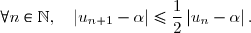
} \\\overset{\phantom{.}}{\phantom{1\le\alpha\le2\quad}\Longrightarrow\quad|1-\alpha|\le1} \\\overset{\phantom{.}}{\phantom{1\le\alpha\le2\quad}\Longrightarrow\quad\boxed{|u_0-\alpha|\le1}})

\ge\ln(10^3)} \\\overset{\phantom{.}}{\phantom{\dfrac{1}{2^n}\le10^{-3}\quad}\Longleftrightarrow\quad n\times\ln2\ge3\times\ln10})

 définie sur ]-a ; a ] par
 =(x+a)-\ln(x+a).)
=1-\dfrac{1}{x+a}\quad\Longrightarrow\quad\boxed{\Delta'(x)=\dfrac{x+a-1}{x+a}})
=1-\ln1=1 \end{matrix}{\white{www}}\begin{matrix}|\\|\\|\\|\\|\\|\\|\\|\\|\\|\\|\end{matrix}{\white{www}}\begin{matrix} \begin{array}{|c|ccccccc|}\hline &&&&&&&\\ x&-a&&1-a&&0&&a\\&&&&&&&\\\hline &&&&&&&\\x+a-1&-&-&0&+&+&+&+\\x+a&0&+&+&+&+&+&+\\&&&&&&&\\\hline&||&&&&&&\\\Delta'(x)&||&-&0&+&+&+&+\\&||&&&&&&\\\hline&||&&&&&&\\\Delta(x)&||&\searrow&&\nearrow&\nearrow&\nearrow&\\&||&&1&&&&\\ \hline \end{array}\end{matrix})
![A(a)= \begin{aligned}\int\nolimits_{0}^{a} \left(\overset{}{x+a-\ln(x+a)}\right)\,\text d x\end{aligned} \\\\\phantom{A(a)}= \begin{aligned}\int\nolimits_{0}^{a} \left(\overset{}{x+a}\right)\,\text d x\end{aligned}-\begin{aligned}\int\nolimits_{0}^{a} \ln(x+a)\,\text d x\end{aligned} \\\\\text{Or } \begin{aligned}\int\nolimits_{0}^{a} \left(\overset{}{x+a}\right)\,\text d x\end{aligned}= \left[\overset{}{\dfrac{(x+a)^2}{2}}\right]_0^a=\dfrac{(a+a)^2}{2}-\dfrac{(0+a)^2}{2} \\\phantom{WWWWWWW1}=\dfrac{4a^2}{2}-\dfrac{a^2}{2}=\dfrac{3a^2}{2} \\\\\phantom{\text{Or } }\Longrightarrow\boxed{\begin{aligned}\int\nolimits_{0}^{a} \left(\overset{}{x+a}\right)\,\text d x\end{aligned}=\dfrac{3a^2}{2}}](https://latex.ilemaths.net/latex-0.tex?A(a)= \begin{aligned}\int\nolimits_{0}^{a} \left(\overset{}{x+a-\ln(x+a)}\right)\,\text d x\end{aligned} \\\\\phantom{A(a)}= \begin{aligned}\int\nolimits_{0}^{a} \left(\overset{}{x+a}\right)\,\text d x\end{aligned}-\begin{aligned}\int\nolimits_{0}^{a} \ln(x+a)\,\text d x\end{aligned} \\\\\text{Or } \begin{aligned}\int\nolimits_{0}^{a} \left(\overset{}{x+a}\right)\,\text d x\end{aligned}= \left[\overset{}{\dfrac{(x+a)^2}{2}}\right]_0^a=\dfrac{(a+a)^2}{2}-\dfrac{(0+a)^2}{2} \\\phantom{WWWWWWW1}=\dfrac{4a^2}{2}-\dfrac{a^2}{2}=\dfrac{3a^2}{2} \\\\\phantom{\text{Or } }\Longrightarrow\boxed{\begin{aligned}\int\nolimits_{0}^{a} \left(\overset{}{x+a}\right)\,\text d x\end{aligned}=\dfrac{3a^2}{2}})
![\text{Calculons par parties, }\begin{aligned}\int\nolimits_{0}^{a} \ln(x+a)\,\text d x\end{aligned} =\begin{aligned}\int\nolimits_{0}^{a} 1\times\ln(x+a)\,\text d x\end{aligned} \\\\\underline{\text{Formule de l'intégrale par parties}}\ :\ {\blue{\begin{aligned}\int\nolimits_{0}^{a} u(x)v'(x)\,\text d x\end{aligned}=\left[\overset{}{u(x)v(x)}\right]\limits_0^{a}-\begin{aligned}\int\nolimits_{0}^{a} u'(x)v(x)\,\text d x\end{aligned}}}. \\\\\left\lbrace\begin{matrix}u(x)=\ln(x+a)\phantom{www}\Longrightarrow\phantom{ww}u'(x)=\dfrac{1}{x+a}\\v'(x)=1\phantom{wwwwwwwv}\Longrightarrow\quad v(x)=x+a\phantom{ww}\end{matrix}\right.](https://latex.ilemaths.net/latex-0.tex?\text{Calculons par parties, }\begin{aligned}\int\nolimits_{0}^{a} \ln(x+a)\,\text d x\end{aligned} =\begin{aligned}\int\nolimits_{0}^{a} 1\times\ln(x+a)\,\text d x\end{aligned} \\\\\underline{\text{Formule de l'intégrale par parties}}\ :\ {\blue{\begin{aligned}\int\nolimits_{0}^{a} u(x)v'(x)\,\text d x\end{aligned}=\left[\overset{}{u(x)v(x)}\right]\limits_0^{a}-\begin{aligned}\int\nolimits_{0}^{a} u'(x)v(x)\,\text d x\end{aligned}}}. \\\\\left\lbrace\begin{matrix}u(x)=\ln(x+a)\phantom{www}\Longrightarrow\phantom{ww}u'(x)=\dfrac{1}{x+a}\\v'(x)=1\phantom{wwwwwwwv}\Longrightarrow\quad v(x)=x+a\phantom{ww}\end{matrix}\right. )
![\text{Dès lors, }\ \begin{aligned}\int\nolimits_{0}^{a} \ln(x+a)\,\text d x\end{aligned}=\left[\overset{}{(x+a)\times\ln(x+a)}\right]\limits_0^{a}- \begin{aligned}\int\nolimits_0^{a}\dfrac{1}{x+a}\times(x+a)\,\text d x\end{aligned} \\\\\phantom{WWWWWWWWxWW}=\left[\overset{}{(x+a)\times\ln(x+a)}\right]\limits_0^{a}- \begin{aligned}\int\nolimits_0^{a}1\,\text d x\end{aligned}](https://latex.ilemaths.net/latex-0.tex?\text{Dès lors, }\ \begin{aligned}\int\nolimits_{0}^{a} \ln(x+a)\,\text d x\end{aligned}=\left[\overset{}{(x+a)\times\ln(x+a)}\right]\limits_0^{a}- \begin{aligned}\int\nolimits_0^{a}\dfrac{1}{x+a}\times(x+a)\,\text d x\end{aligned} \\\\\phantom{WWWWWWWWxWW}=\left[\overset{}{(x+a)\times\ln(x+a)}\right]\limits_0^{a}- \begin{aligned}\int\nolimits_0^{a}1\,\text d x\end{aligned})
![\\\\\phantom{WWWWWWWWxWW}=\left[\overset{}{(x+a)\times\ln(x+a)}\right]\limits_0^{a}- \left[\overset{{\white{\frac{}{}}}}{x}\right]\limits_0^{a} \\\overset{\phantom{.}}{\phantom{WWWWWWWWxWW}=[2a\ln(2a)-a\ln a]-(a-0)} \\\overset{\phantom{.}}{\phantom{WWWWWWWWxWW}=2a\ln(2a)-a\ln a-a} \\\overset{\phantom{.}}{\phantom{WWWWWWWWxWW}=a[2\ln(2a)-\ln a-1]} \\\overset{\phantom{.}}{\phantom{WWWWWWWWxWW}=a[\ln(2a)^2-\ln a-1]} \\\overset{\phantom{.}}{\phantom{WWWWWWWWxWW}=a[\ln(4a^2)-\ln a-1]} \\\overset{\phantom{.}}{\phantom{WWWWWWWWxWW}=a[\ln\dfrac{4a^2}{a}-1]} \\\overset{\phantom{.}}{\phantom{WWWWWWWWxWW}=a[\ln(4a)-1]} \\\\\Longrightarrow\boxed{\begin{aligned}\int\nolimits_{0}^{a} \ln(x+a)\,\text d x\end{aligned}=a[\ln(4a)-1]}](https://latex.ilemaths.net/latex-0.tex?\\\\\phantom{WWWWWWWWxWW}=\left[\overset{}{(x+a)\times\ln(x+a)}\right]\limits_0^{a}- \left[\overset{{\white{\frac{}{}}}}{x}\right]\limits_0^{a} \\\overset{\phantom{.}}{\phantom{WWWWWWWWxWW}=[2a\ln(2a)-a\ln a]-(a-0)} \\\overset{\phantom{.}}{\phantom{WWWWWWWWxWW}=2a\ln(2a)-a\ln a-a} \\\overset{\phantom{.}}{\phantom{WWWWWWWWxWW}=a[2\ln(2a)-\ln a-1]} \\\overset{\phantom{.}}{\phantom{WWWWWWWWxWW}=a[\ln(2a)^2-\ln a-1]} \\\overset{\phantom{.}}{\phantom{WWWWWWWWxWW}=a[\ln(4a^2)-\ln a-1]} \\\overset{\phantom{.}}{\phantom{WWWWWWWWxWW}=a[\ln\dfrac{4a^2}{a}-1]} \\\overset{\phantom{.}}{\phantom{WWWWWWWWxWW}=a[\ln(4a)-1]} \\\\\Longrightarrow\boxed{\begin{aligned}\int\nolimits_{0}^{a} \ln(x+a)\,\text d x\end{aligned}=a[\ln(4a)-1]})
![A(a)= \begin{aligned}\int\nolimits_{0}^{a} \left(\overset{}{x+a}\right)\,\text d x\end{aligned}-\begin{aligned}\int\nolimits_{0}^{a} \ln(x+a)\,\text d x\end{aligned} \\\overset{{\phantom{.}}}{\phantom{A(a)}= \dfrac{3a^2}{2}-a[\ln(4a)-1]} \\\\\Longrightarrow\boxed{A(a)= \dfrac{3a^2}{2}-a[\ln(4a)-1]}](https://latex.ilemaths.net/latex-0.tex?A(a)= \begin{aligned}\int\nolimits_{0}^{a} \left(\overset{}{x+a}\right)\,\text d x\end{aligned}-\begin{aligned}\int\nolimits_{0}^{a} \ln(x+a)\,\text d x\end{aligned} \\\overset{{\phantom{.}}}{\phantom{A(a)}= \dfrac{3a^2}{2}-a[\ln(4a)-1]} \\\\\Longrightarrow\boxed{A(a)= \dfrac{3a^2}{2}-a[\ln(4a)-1]})
![{\red{2.\;}}\;A\left(\dfrac{\text{e}^2}{4}\right)=\dfrac{3\left(\frac{\text{e}^2}{4}\right)^2}{2}-\left(\dfrac{\text{e}^2}{4}\right)[\ln(4\times\left(\frac{\text{e}^2}{4}\right))-1] \\\\\phantom{{\red{2.\;}}\;A\left(\dfrac{\text{e}^2}{4}\right)}=\dfrac{3\left(\frac{\text{e}^4}{16}\right)}{2}-\left(\dfrac{\text{e}^2}{4}\right)[\ln(\text{e}^2)-1] \\\\\phantom{{\red{2.\;}}\;A\left(\dfrac{\text{e}^2}{4}\right)}=\dfrac{3\text{e}^4}{32}-\left(\dfrac{\text{e}^2}{4}\right)[2-1] \\\\\phantom{{\red{2.\;}}\;A\left(\dfrac{\text{e}^2}{4}\right)}=\dfrac{3\text{e}^4}{32}-\dfrac{\text{e}^2}{4} \\\\\phantom{{\red{2.\;}}\;A\left(\dfrac{\text{e}^2}{4}\right)}=\dfrac{\text{e}^2}{4}\left(\dfrac{3\text{e}^2}{8}-1\right) \\\\\Longrightarrow\boxed{A\left(\dfrac{\text{e}^2}{4}\right)=\dfrac{\text{e}^2}{4}\left(\dfrac{3\text{e}^2}{8}-1\right)}](https://latex.ilemaths.net/latex-0.tex?{\red{2.\;}}\;A\left(\dfrac{\text{e}^2}{4}\right)=\dfrac{3\left(\frac{\text{e}^2}{4}\right)^2}{2}-\left(\dfrac{\text{e}^2}{4}\right)[\ln(4\times\left(\frac{\text{e}^2}{4}\right))-1] \\\\\phantom{{\red{2.\;}}\;A\left(\dfrac{\text{e}^2}{4}\right)}=\dfrac{3\left(\frac{\text{e}^4}{16}\right)}{2}-\left(\dfrac{\text{e}^2}{4}\right)[\ln(\text{e}^2)-1] \\\\\phantom{{\red{2.\;}}\;A\left(\dfrac{\text{e}^2}{4}\right)}=\dfrac{3\text{e}^4}{32}-\left(\dfrac{\text{e}^2}{4}\right)[2-1] \\\\\phantom{{\red{2.\;}}\;A\left(\dfrac{\text{e}^2}{4}\right)}=\dfrac{3\text{e}^4}{32}-\dfrac{\text{e}^2}{4} \\\\\phantom{{\red{2.\;}}\;A\left(\dfrac{\text{e}^2}{4}\right)}=\dfrac{\text{e}^2}{4}\left(\dfrac{3\text{e}^2}{8}-1\right) \\\\\Longrightarrow\boxed{A\left(\dfrac{\text{e}^2}{4}\right)=\dfrac{\text{e}^2}{4}\left(\dfrac{3\text{e}^2}{8}-1\right)}) Publié par malou
le
Publié par malou
le
 Voir l'énoncé seul
 forum de terminale