1. Soit un nombre rationnel strictement positif et un entier naturel.
1. a) Nous devons calculer
Soit la fonction définie sur par
Nous obtenons alors :
1. b) Nous devons calculer
Soit la fonction définie sur par
Nous obtenons alors :
2. a) Une primitive de la fonction est la fonction où est un nombre réel constant.
2. b) Une primitive de la fonction est la fonction où est un nombre réel constant et
4 points
exercice 2
Soit le polynôme défini par
1. Montrons que 1 est racine de
Donc 1 est racine de
Montrons que est racine de
Donc est racine de
2. Nous devons déterminer le polynôme tel que
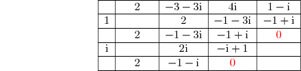
Déterminons le polynôme en appliquant deux fois la méthode de Horner.
Nous en déduisons que et par conséquent
3. Nous devons résoudre dans l'équation
D'où l'ensemble des solutions de l'équation est
4. On pose et
4. a) Représentation graphique des points A, B et C (voir question 5.)
4. b)Montrons que le point C est le milieu du segment [AB ].
Par conséquent, le point C est le milieu du segment [AB ].
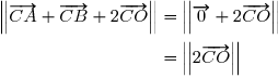
Montrons que le point C appartient à l'ensemble (E ) des points M tels que
Nous devons donc montrer que
Nous savons que le point C est le milieu du segment [AB ] et par suite que
Dès lors,
Nous en déduisons que le point C appartient à l'ensemble (E ).
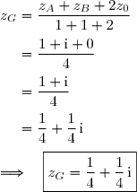
4. c) Nous devons déterminer l'affixe du point G barycentre du système
Représentation graphique du point G (voir question 5).
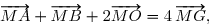
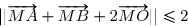
5. Nous devons déterminer et construire l'ensemble (E ) des points M tels que
Le point G est le barycentre du système
Dès lors, pour tout point M du plan, nous obtenons : soit
Dès lors,
Il s'ensuit que M appartient au disque centré en G et de rayon
Par conséquent, l'ensemble (E ) des points M tels que
est le disque centré en G et de rayon
Représentons graphiquement les résultats.
6. L'objectif du jeune agriculteur est de pratiquer sa culture sous serre dans l'ensemble (E ) qui contient un point du segment [AB ].
Son objectif sera atteint s'il pratique sa culture dans un disque de son champ (E ) qui contient le point C milieu du segment [AB ] où les affixes des points A et B sont respectivement et .
4 points
exercice 3
On considère la suite numérique définie par :
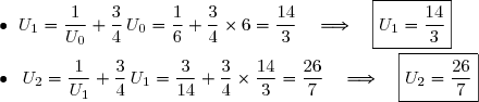
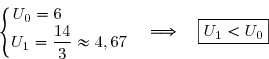
1. Nous devons déterminer et
2. Nous devons démontrer par récurrence que :
Initialisation : Montrons que la propriété est vraie pour n = 0, soit que
C'est une évidence car
Donc l'initialisation est vraie.
Hérédité : Montrons que si pour un nombre naturel n fixé, la propriété est vraie au rang n , alors elle est encore vraie au rang (n +1).
Montrons donc que si pour un nombre naturel n fixé, , alors nous obtenons , soit
Nous observons que
Dès lors,
Par conséquent,
Donc l'hérédité est vraie.
Puisque l'initialisation et l'hérédité sont vraies, nous avons montré par récurrence que
3. Soit la fonction définie sur par
3. a) Nous devons étudier le sens de variations de
La fonction est dérivable sur
Nous savons que car .
De plus,
Il s'ensuit que le signe de est le signe de
Tableau de signes de
D'où le tableau de variations de
Par conséquent, est strictement décroissante sur et strictement croissante sur
3. b) Nous devons en déduire par récurrence que est strictement décroissante.
Initialisation : Montrons que
C'est une évidence car
Donc l'initialisation est vraie.
Hérédité : Montrons que si pour un nombre naturel n fixé, la propriété est vraie au rang n , alors elle est encore vraie au rang (n +1).
Montrons donc que si pour un nombre naturel n fixé, , alors nous obtenons
Dans la question 2., nous avons montré que :
Puisque nous en déduisons que et par suite
Dès lors, et
De plus, nous savons que est strictement croissante sur
D'où, en utilisant l'hypothèse de récurrence, nous obtenons :
Donc l'hérédité est vraie.
Puisque l'initialisation et l'hérédité sont vraies, nous avons montré par récurrence que est strictement décroissante.
4. Dans les questions 2. et 3. b), nous avons montré que la suite est décroissante et minorée par .
Nous en déduisons que la suite est convergente.
Déterminons sa limite.
La fonction f est continue sur
La suite (Un ) est définie par la relation de récurrence :
Nous savons que la suite (Un ) est convergente vers .
Selon le théorème du point fixe, nous déduisons que vérifie la relation
Or
Donc
Par conséquent,
9 points
probleme
Partie A (2 points)
On considère l'équation différentielle
1. Nous devons résoudre l'équation différentielle
La solution générale d'une équation différentielle de la forme est
Dans ce cas, a = -2 et b = 0.
D'où la solution générale de l'équation s'écrit
2. Soit une fonction définie sur par où et sont des réels.
Nous devons déterminer et pour que soit une solution de
La fonction est dérivable sur
Pour tout
est une solution de
3. a) Soit une fonction dérivable sur
Posons et
Donc
Rappel : Nous avons montré dans la question 2 que pour les valeurs et la fonction est une solution de
Nous devons démontrer que est une solution de si et seulement si est une solution de
est une solution de est une solution de
Par conséquent, est une solution de si et seulement si est une solution de
3. b) Nous devons en déduire l'ensemble des solutions de
Nous savons que est une solution de si et seulement si est une solution de soit
D'où l'ensemble des solutions de est l'ensemble des fonctions définies sur par
4. Déterminons la solution de dont la courbe représentative passe par le point
Par conséquent,
Partie B (7 points)
Soit la fonction définie par
1. La fonction est partout définie sauf si La fonction est donc définie sur l'ensemble des réels différents de 1.
D'où l'ensemble de définition de est
2. Étudions les limites de aux bornes de
Calculons
Par conséquent,
Calculons
Remarque :
Si tend vers +, alors x est supérieur à 1 et donc
Nous obtenons alors :
Par conséquent,
Dès lors, en +, la courbe admet une asymptote horizontale d'équation
Calculons
Nous en déduisons que :
Par conséquent, la droite d'équation est une asymptote verticale à la courbe
3. Déterminons
Si tend vers -, alors x est inférieur à 0.
Nous obtenons alors :
Nous en déduisons que :
Par conséquent, en -, la courbe admet une branche parabolique de direction l'axe des ordonnées.
4. Étudions la continuité de en 0.
D'une part,
D'autre part,
D'où
Par conséquent, nous obtenons :
Donc la fonction est continue en 0.
5. Étudions la dérivabilité de en 0.
Premier cas :
Nous en déduisons que
D'où, est dérivable à gauche en 0 et
Second cas :
Dans ce cas, (voir question 2 - Partie B)
Nous obtenons alors :
Nous en déduisons que
D'où, est dérivable à droite en 0 et
Puisque les nombres dérivés à gauche et à droite de sont des nombres réels différents, nous en déduisons que la fonction n'est pas dérivable en 0.
Il s'ensuit graphiquement que la courbe admet un point anguleux de coordonnées (0 ; 0). De plus, au point de coordonnées (0 ; 0), la courbe admet une demi-tangente à gauche de coefficient directeur égal à 10 et une demi-tangente à droite de coefficient directeur égal à 0 (demi-tangente horizontale).
6.Calculons sur
Calculons sur
Étudions le signe de
Par conséquent,
Puisque le signe de est le signe de
7. Dressons le tableau de variations de
8. Montrons que sur l'intervalle ]1 ; 2[ l'équation admet une unique solution et que
La fonction f est continue et strictement décroissante sur
Il s'ensuit que f réalise une bijection de sur
Or
Dès lors, l'équation admet une unique solution sur
Par conséquent, sur l'intervalle ]1 ; 2[ l'équation admet une unique solution et
9. Représentation graphique de et de ses asymptotes.
10) Nous devons calculer en cm2 l'aire de la partie du plan comprise entre les droites d'équations et
la courbe de
Notons que si car
Sur l'intervalle [2 ; 3], la courbe est au-dessus de la droite d'équation
Nous obtenons alors :
Or l'unité graphique est 2 cm.
Donc l'unité d'aire (u. a.) est 4 cm2.
Par conséquent,
Publié par malou/Panter
le
ceci n'est qu'un extrait
Pour visualiser la totalité des cours vous devez vous inscrire / connecter (GRATUIT) Inscription Gratuitese connecter
Merci à Hiphigenie / malou pour avoir contribué à l'élaboration de cette fiche
Désolé, votre version d'Internet Explorer est plus que périmée ! Merci de le mettre à jour ou de télécharger Firefox ou Google Chrome pour utiliser le site. Votre ordinateur vous remerciera !

 un nombre rationnel strictement positif et
  un entier naturel.
}{x}.)
 définie sur
 ![\overset{ { \white{ . } } } { ]\,-1\;;\;+\infty[}](https://latex.ilemaths.net/latex-0.tex?\overset{ { \white{ . } } } { ]\,-1\;;\;+\infty[}) par
par =\ln(x+1).} )

}{x}=\lim\limits_{x\to 0}\dfrac{\ln(x+1)-\ln(0+1)}{x-0} \\\overset{ { \white{ . } } } {\phantom{\lim\limits_{x\to 0}\dfrac{\ln(x+1)}{x}}=\lim\limits_{x\to 0}\dfrac{f(x)-f(0)}{x-0}} \\\overset{ { \white{ . } } } {\phantom{\lim\limits_{x\to 0}\dfrac{\ln(x+1)}{x}}=f'(0)} \\\\\text{Or }\;f(x)=\ln(x+1) \quad\Longrightarrow\quad f'(x)=\dfrac{1}{x+1} \\\overset{ { \white{ . } } } {\phantom{WWWWWWWWi}\quad\Longrightarrow\quad f'(0)=1} \\\\\Longrightarrow\quad\boxed{\lim\limits_{x\to 0}\dfrac{\ln(x+1)}{x}=1})

 définie sur
  par
par =\text e^x.} )
-g(0)}{x-0}} \\\overset{ { \white{ . } } } {\phantom{\lim\limits_{x\to 0}\dfrac{\text e^x-1}{x}}=g'(0)} \\\\\text{Or }\;g(x)=\text e^x \quad\Longrightarrow\quad g'(x)=\text e^x \\\overset{ { \white{ . } } } {\phantom{WWWWWi}\quad\Longrightarrow\quad g'(0)=\text e^0=1} \\\\\Longrightarrow\quad\boxed{\lim\limits_{x\to 0}\dfrac{\text e^x-1}{x}=1} )
(x)f'(x)}) est la fonction
est la fonction (x)+c}) où
où  est un nombre réel constant.
}{f(x)}}) est la fonction
est la fonction \right|)+c}) où
où \neq0. } )
 défini par
 =2z^3-3(1+\text i)z^2+4\text iz+1-\text i\quad\text{où }\;z\in\C.} )

=2\times 1^3-3(1+\text i)\times 1^2+4\text i\times1+1-\text i \\\overset{ { \white{ . } } } {\phantom{P(1)}=2-3(1+\text i)+4\text i+1-\text i} \\\overset{ { \white{ . } } } {\phantom{P(1)}=2-3-3\text i+4\text i+1-\text i} \\\overset{ { \white{ . } } } {\phantom{P(1)}=0} \\\\\Longrightarrow\boxed{P(1)=0})
 est racine de
 =2\times \text i^3-3(1+\text i)\times \text i^2+4\text i\times\text i+1-\text i \\\overset{ { \white{ . } } } {\phantom{P(1)}=2\times(-\text i)-3(1+\text i)\times(-1)+4\text i^2+1-\text i} \\\overset{ { \white{ . } } } {\phantom{P(1)}=-2\text i+3(1+\text i)-4+1-\text i} \\\overset{ { \white{ . } } } {\phantom{P(1)}=-2\text i+3+3\text i-4+1-\text i} \\\overset{ { \phantom{ . } } } {\phantom{P(1)}=0} \\\\\Longrightarrow\boxed{P(\text i)=0})
 est racine de
 =(z-1)(z-\text i)g(z). } )
=2z-1-\text i} } ) et par conséquent
et par conséquent =(z-1)(z-\text i)(2z-1-\text i)}. } )
 l'équation
 =0. } )
=0\quad\Longleftrightarrow\quad (z-1)(z-\text i)(2z-1-\text i)=0 \\\overset{ { \white{ . } } } {\phantom{P(z)=0}\quad\Longleftrightarrow\quad z-1=0\quad\text{ou}\quad z-\text i=0\quad\text{ou}\quad 2z-1-\text i=0} \\\overset{ { \white{ . } } } {\phantom{P(z)=0}\quad\Longleftrightarrow\quad z=1\quad\text{ou}\quad z=\text i\quad\text{ou}\quad 2z=1+\text i} \\\overset{ { \white{ . } } } {\phantom{P(z)=0}\quad\Longleftrightarrow\quad \boxed{z=1\quad\text{ou}\quad z=\text i\quad\text{ou}\quad z=\dfrac 1 2+\dfrac 1 2\,\text i}})
=0 } ) est
est 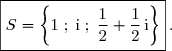
 et
et 
 Montrons que le point C est le milieu du segment [AB ].
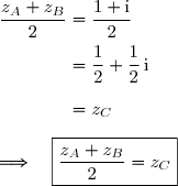

^2+\left(\dfrac 1 2 \right)^2}} \\\overset{ { \white{ . } } } {\phantom{||\overrightarrow{CA}+\overrightarrow{CB}+2\overrightarrow{CO}||}=2\,\sqrt{\dfrac 1 4+\dfrac 1 4}} \\\overset{ { \white{ . } } } {\phantom{||\overrightarrow{CA}+\overrightarrow{CB}+2\overrightarrow{CO}||}=2\,\sqrt{\dfrac 2 4}})

 du point G barycentre du système
 \;;\;(B,1)\;;\;(O,2)\rbrace.} )
\overrightarrow{MG},} )


 est le disque centré en G et de rayon
 et
et  .
._{n\in\N} } ) définie par :
définie par : }\end{matrix}\right. } )
 et
et 

 , alors nous obtenons
  , soit
^2-4\sqrt 3\,U_n+4}{4\,U_n}} \\\overset{ { \white{ . } } } {\phantom{U_{n+1}-\sqrt 3}=\dfrac{(\sqrt 3\,U_n-2)^2}{4\,U_n}})
^2\ge 0\phantom{WWWWWWWWWWW}\\\overset{ { \white{ . } } } {U_n\ge\sqrt 3\quad\Longrightarrow\quad U_n>0\quad\Longrightarrow\quad 4U_n>0}\end{matrix}\right. } )
^2}{4\,U_n}\ge 0. } )

 la fonction définie sur
 ![\overset{ { \white{ . } } } {]\,0\;;\;+\infty\,[ }](https://latex.ilemaths.net/latex-0.tex?\overset{ { \white{ . } } } {]\,0\;;\;+\infty\,[ } ) par
par =\dfrac 1 x + \dfrac 3 4 x.} )

![\overset{ { \white{ . } } } {]\,0\;;\;+\infty\,[\,. }](https://latex.ilemaths.net/latex-0.tex?\overset{ { \white{ . } } } {]\,0\;;\;+\infty\,[\,. } )
![\forall\,x\in\,]\,0\;;\;+\infty\,[\,,\;f'(x)=-\dfrac{1}{x^2}+\dfrac 3 4 \\\overset{ { \white{ . } } } {\phantom{\forall\,x\in\,]\,0\;;\;+\infty\,[\,,\;f'(x)}=\dfrac{-4+3x^2}{4x^2}} \\\overset{ { \white{ . } } } {\phantom{\forall\,x\in\,]\,0\;;\;+\infty\,[\,,\;f'(x)}=\dfrac{3x^2-4}{4x^2}} \\\overset{ { \white{ . } } } {\phantom{\forall\,x\in\,]\,0\;;\;+\infty\,[\,,\;f'(x)}=\dfrac{(\sqrt 3\,x+2)(\sqrt 3\,x-2)}{4x^2}} \\\\\Longrightarrow\quad\boxed{\forall\,x\in\,]\,0\;;\;+\infty\,[\,,\;f'(x)=\dfrac{(\sqrt 3\,x+2)(\sqrt 3\,x-2)}{4x^2}}](https://latex.ilemaths.net/latex-0.tex?\forall\,x\in\,]\,0\;;\;+\infty\,[\,,\;f'(x)=-\dfrac{1}{x^2}+\dfrac 3 4 \\\overset{ { \white{ . } } } {\phantom{\forall\,x\in\,]\,0\;;\;+\infty\,[\,,\;f'(x)}=\dfrac{-4+3x^2}{4x^2}} \\\overset{ { \white{ . } } } {\phantom{\forall\,x\in\,]\,0\;;\;+\infty\,[\,,\;f'(x)}=\dfrac{3x^2-4}{4x^2}} \\\overset{ { \white{ . } } } {\phantom{\forall\,x\in\,]\,0\;;\;+\infty\,[\,,\;f'(x)}=\dfrac{(\sqrt 3\,x+2)(\sqrt 3\,x-2)}{4x^2}} \\\\\Longrightarrow\quad\boxed{\forall\,x\in\,]\,0\;;\;+\infty\,[\,,\;f'(x)=\dfrac{(\sqrt 3\,x+2)(\sqrt 3\,x-2)}{4x^2}})
 car
car ![\overset{ { \white{ . } } } {x\in\;]0\;;\;+\infty[ }](https://latex.ilemaths.net/latex-0.tex?\overset{ { \white{ . } } } {x\in\;]0\;;\;+\infty[ } ) .
.
 } ) est le signe de
est le signe de 
. } )
&||&-&0&+ &\\&||&&&&\\\hline \end{array})

&||&-&0&+ &\\&||&&&&\\\hline &||&&&&\\f&||&\searrow&&\nearrow &\\&||&&f\left(\dfrac {2 \sqrt{3}}{3}\right)&&\\\hline \end{array})
![\left]\,0\;;\;\dfrac {2 \sqrt{3}}{3}\right]](https://latex.ilemaths.net/latex-0.tex?\left]\,0\;;\;\dfrac {2 \sqrt{3}}{3}\right]) et strictement croissante sur
et strictement croissante sur 

 , alors nous obtenons
 nous en déduisons que
  et par suite
 et
et 
<f\left(U_{n}\right) \\\overset{ { \white{ . } } } {\phantom{ U_{n+1}<U_n}\quad\Longrightarrow\quad \boxed{ U_{n+2}<U_{n+1}}}\quad\quad\text{car }\left\lbrace\begin{matrix}f\left(U_{n+1}\right)=U_{n+2}\\f\left(U_{n}\right)=U_{n+1}\end{matrix}\right.)
_{n\in\N}}) est décroissante et minorée par
est décroissante et minorée par  .
..})
 .
..})
\quad\Longleftrightarrow\quad\ell=\dfrac 1\ell+\dfrac 34\, \ell \\\overset{{\white{.}}}{\phantom{\ell=f(\ell)}\quad\Longleftrightarrow\quad\ell=\dfrac {4+3\,\ell^2}{4\,\ell}} \\\overset{{\white{.}}}{\phantom{\ell=f(\ell)}\quad\Longleftrightarrow\quad 4\,\ell^2=4+3\,\ell^2} \\\overset{{\white{.}}}{\phantom{\ell=f(\ell)}\quad\Longleftrightarrow\quad 4\,\ell^2-3\,\ell^2=4} \\\overset{{\phantom{.}}}{\phantom{\ell=f(\ell)}\quad\Longleftrightarrow\quad \ell^2=4} \\\overset{{\phantom{.}}}{\phantom{\ell=f(\ell)}\quad\Longleftrightarrow\quad \ell=2\quad\text{ou}\quad\ell=-2})


:\dfrac 1 2 y'+y=3\,\text e^{-2x}+2. } )
:\dfrac 1 2 y'+y=0. } )
 est
est .)

}) s'écrit
s'écrit =c\,\text{e}^{-2x}\ \ (c\in\R)})
 une fonction définie sur
  par
par =ax\,\text e^{-2x}+b } ) où
où  et
et  sont des réels.
 pour que
  soit une solution de
 . } )


=(ax)'\times\,\text e^{-2x}+ax\times(\text e^{-2x})' \\\overset{ { \white{ . } } } { \phantom{h'(x)}=a\times\text e^{-2x}+ax\times(-2\text e^{-2x})} \\\\\Longrightarrow\quad\boxed{h'(x)=a\,\text e^{-2x}-2ax\,\text e^{-2x}})
\quad\Longleftrightarrow\quad \dfrac 1 2 h'(x)+h(x)=3\,\text e^{-2x}+2} )

+(ax\,\text e^{-2x}+b )=3\,\text e^{-2x}+2} \\\overset{ { \white{ . } } } { \Longleftrightarrow\quad \dfrac 1 2 a\,\text e^{-2x}-ax\,\text e^{-2x}+ax\,\text e^{-2x}+b =3\,\text e^{-2x}+2} \\\overset{ { \white{ . } } } { \Longleftrightarrow\quad \dfrac 1 2 a\,\text e^{-2x}+b =3\,\text e^{-2x}+2})
 une fonction dérivable sur
 et
et 
=6x\,\text e^{-2x}+2. } )
 et
et  la fonction
 .})
 } ) si et seulement si
si et seulement si  est une solution de
 . } )
 est une solution de
 \quad\Longleftrightarrow\quad\dfrac 1 2 \Big(g(x)-h(x)\Big)'+\Big(g(x)-h(x)\Big)=0 } )

-\dfrac 1 2\,h'(x)+g(x)-h(x)=0 } \\\overset{ { \white{ . } } } {\quad\Longleftrightarrow\quad\dfrac 1 2\,g'(x)+g(x)=\dfrac 1 2\,h'(x)+h(x) } \\\overset{ { \white{ . } } } {\quad\Longleftrightarrow\quad\dfrac 1 2\,g'(x)+g(x)=3\,\text e^{-2x}+2} \\\phantom{WWWWWWWWWW}\quad\text{car }h\,\text{est une solution de }(E) )

 est une solution de
 })
. } )
, } ) soit
soit -h(x)=c\,\text{e}^{-2x}\ \ (c\in\R). } )
-h(x)=c\,\text{e}^{-2x}\ \ (c\in\R)\quad\Longleftrightarrow\quad g(x)=h(x)+c\,\text{e}^{-2x}\ \ (c\in\R) } \\\overset{ { \white{ . } } } { \phantom{WWWWWWWWWWwWWW} \quad\Longleftrightarrow\quad g(x)=6x\,\text e^{-2x}+2 +c\,\text{e}^{-2x}\ \ (c\in\R) } \\\overset{ { \white{ . } } } { \phantom{WWWWWWWWWWwWWW} \quad\Longleftrightarrow\quad \boxed {g(x)=(6x+c)\,\text e^{-2x}+2 \ \ (c\in\R) } })
 par
par =(6x+c)\,\text e^{-2x}+2 \ \ (c\in\R). } )
 de
de  } ) passe par le point
passe par le point  .} )
\in(\mathscr{C}_k)\quad\Longleftrightarrow\quad k(0)=0 \\\overset{ { \white{ _. } } } {\phantom{WWWWWWv} \quad\Longleftrightarrow\quad(0+c)\,\text e^{0}+2=0} \\\overset{ { \white{ _. } } } {\phantom{WWWWWWv} \quad\Longleftrightarrow\quad c+2=0} \\\overset{ { \phantom{ _. } } } {\phantom{WWWWWWv} \quad\Longleftrightarrow\quad c=-2})
=(6x-2)\,\text e^{-2x}+2 }\,.})
 définie par
 =\left\lbrace\begin{matrix}(6x-2)\,\text e^{-2x}+2\quad\text{si }x\le0\\\dfrac{x+\ln|1-x|}{1-x}\quad\quad\;\text{si }x>0\end{matrix}\right. })

 La fonction

.})
![\lim\limits_{x\to-\infty}f(x)=\lim\limits_{x\to-\infty}[(6x-2)\,\text e^{-2x}+2] \\\\\text{Or }\;\left\lbrace\begin{matrix}\lim\limits_{x\to-\infty}(6x-2)=-\infty\phantom{WWWWWWWWWWW}\\\left.\begin{matrix}\lim\limits_{x\to-\infty}(-2x)=+\infty\\\lim\limits_{X\to+\infty}\text e^X=+\infty\end{matrix}\right\rbrace\quad\underset{(X=-2x)}{\Longrightarrow}\quad\lim\limits_{x\to-\infty}\text e^{-2x}=+\infty \end{matrix}\right. \\\\\text{D'où }\;\lim\limits_{x\to-\infty}(6x-2)\,\text e^{-2x}=-\infty \\\\\text{et }\lim\limits_{x\to-\infty}[(6x-2)\,\text e^{-2x}+2]=+\infty](https://latex.ilemaths.net/latex-0.tex?\lim\limits_{x\to-\infty}f(x)=\lim\limits_{x\to-\infty}[(6x-2)\,\text e^{-2x}+2] \\\\\text{Or }\;\left\lbrace\begin{matrix}\lim\limits_{x\to-\infty}(6x-2)=-\infty\phantom{WWWWWWWWWWW}\\\left.\begin{matrix}\lim\limits_{x\to-\infty}(-2x)=+\infty\\\lim\limits_{X\to+\infty}\text e^X=+\infty\end{matrix}\right\rbrace\quad\underset{(X=-2x)}{\Longrightarrow}\quad\lim\limits_{x\to-\infty}\text e^{-2x}=+\infty \end{matrix}\right. \\\\\text{D'où }\;\lim\limits_{x\to-\infty}(6x-2)\,\text e^{-2x}=-\infty \\\\\text{et }\lim\limits_{x\to-\infty}[(6x-2)\,\text e^{-2x}+2]=+\infty)
=-\infty} })
.})
 Si
Si  tend vers +
 , alors x est supérieur à 1 et donc
=\lim\limits_{x\to+\infty}\dfrac{x+\ln(x-1)}{1-x} \\\overset{ { \white{ . } } } {\phantom{\lim\limits_{x\to+\infty}f(x) }=\lim\limits_{x\to+\infty}\left(\dfrac{x}{1-x}+\dfrac{\ln(x-1)}{1-x}\right)} \\\\\text{Or }\;\left\lbrace\begin{matrix}\lim\limits_{x\to+\infty}\dfrac{x}{1-x}=\lim\limits_{x\to+\infty}\dfrac{x}{-x}=-1\phantom{WWWWWWWWWWWWWWWWWWWWWW}\\\\\lim\limits_{x\to+\infty}\dfrac{\ln(x-1)}{1-x}=-\lim\limits_{x\to+\infty}\dfrac{\ln(x-1)}{x-1}\underset{(t=x-1)}{=}-\lim\limits_{t\to+\infty}\dfrac{\ln t}{t}=0\;(\text{croissances comparées})\end{matrix}\right. \\\\\text{D'où }\;\lim\limits_{x\to+\infty}\left(\dfrac{x}{1-x}+\dfrac{\ln(x-1)}{1-x}\right)=-1+0=-1)
=-1} })
 admet une asymptote horizontale d'équation
=\lim\limits_{x\to 1}\dfrac{x+\ln|1-x|}{1-x}.})
=-\infty)
=-\infty\\\overset{ { \white{ . } } } {\lim\limits_{x\to 1^-}(1-x)=0^+\phantom{WWWW}}\\\overset{ { \white{ . } } } {\lim\limits_{x\to 1^+}(1-x)=0^-\phantom{WWWW}}\end{matrix}\right.\quad\Longrightarrow\quad\left\lbrace\begin{matrix}\lim\limits_{x\to 1^-}\dfrac{x+\ln|1-x|}{1-x}=-\infty \\\overset{ { \white{ . } } } {\lim\limits_{x\to 1^+}\dfrac{x+\ln|1-x|}{1-x}=+\infty}\end{matrix}\right. \\\\\phantom{WWWWWWWWWWWW}\quad\Longrightarrow\quad\boxed{\left\lbrace\begin{matrix}\lim\limits_{x\to 1^-}f(x)=-\infty\\\overset{ { \phantom{ . } } } {\lim\limits_{x\to 1^+}f(x)=+\infty}\end{matrix}\right.})
 est une asymptote verticale à la courbe
}{x}\,. })
![\lim\limits_{x\to-\infty} \dfrac{f(x)}{x}=\lim\limits_{x\to-\infty} \dfrac{(6x-2)\,\text e^{-2x}+2}{x} \\\overset{ { \white{ . } } } {\phantom{\lim\limits_{x\to-\infty} \dfrac{f(x)}{x}}=\lim\limits_{x\to-\infty} \left[\left(\dfrac{6x-2}{x}\right)\,\text e^{-2x}+\dfrac{2}{x}\right]}](https://latex.ilemaths.net/latex-0.tex?\lim\limits_{x\to-\infty} \dfrac{f(x)}{x}=\lim\limits_{x\to-\infty} \dfrac{(6x-2)\,\text e^{-2x}+2}{x} \\\overset{ { \white{ . } } } {\phantom{\lim\limits_{x\to-\infty} \dfrac{f(x)}{x}}=\lim\limits_{x\to-\infty} \left[\left(\dfrac{6x-2}{x}\right)\,\text e^{-2x}+\dfrac{2}{x}\right]})
=+\infty\\\lim\limits_{X\to +\infty}\text e^X=+\infty\end{matrix}\right\rbrace\quad\underset{(X=-2x)}{\Longrightarrow}\quad\lim\limits_{x\to -\infty}\text e^{-2x}=+\infty\end{matrix}\right. \\\\\Longrightarrow\lim\limits_{x\to -\infty}\left(\dfrac{6x-2}{x}\right)\,\text e^{-2x}=+\infty)
![\left\lbrace\begin{matrix}\lim\limits_{x\to -\infty}\left(\dfrac{6x-2}{x}\right)\,\text e^{-2x}=+\infty\\\overset{ { \white{ . } } } {\lim\limits_{x\to -\infty}\dfrac{2}{x}=0\phantom{WWWWWWW}}\end{matrix}\right.\quad\Longrightarrow\quad\lim\limits_{x\to -\infty}\left[\left(\dfrac{6x-2}{x}\right)\,\text e^{-2x}+\dfrac 2 x\right]=+\infty\\\\\phantom{WWWWWWWWWWWWW}\quad\Longrightarrow\quad\boxed{\lim\limits_{x\to -\infty}\dfrac{f(x)}{x}=+\infty}](https://latex.ilemaths.net/latex-0.tex?\left\lbrace\begin{matrix}\lim\limits_{x\to -\infty}\left(\dfrac{6x-2}{x}\right)\,\text e^{-2x}=+\infty\\\overset{ { \white{ . } } } {\lim\limits_{x\to -\infty}\dfrac{2}{x}=0\phantom{WWWWWWW}}\end{matrix}\right.\quad\Longrightarrow\quad\lim\limits_{x\to -\infty}\left[\left(\dfrac{6x-2}{x}\right)\,\text e^{-2x}+\dfrac 2 x\right]=+\infty\\\\\phantom{WWWWWWWWWWWWW}\quad\Longrightarrow\quad\boxed{\lim\limits_{x\to -\infty}\dfrac{f(x)}{x}=+\infty})
=(6\times0-2)\,\text e^0+2=-2\times1+2=0\quad\Longrightarrow\quad\boxed{f(0)=0}\,. } )
![\overset{ { \white{ . } } }{\bullet}{\white{x}}\lim\limits_{x\to0^-}\,f(x)=\lim\limits_{x\to0^-}\,\left[(6x-2)\,\text e^{-2x}+2\right]=(6\times0-2)\,\text e^0+2=-2\times1+2=0 \\\\\phantom{W}\Longrightarrow\quad\boxed{\lim\limits_{x\to0^-}\,f(x)=0}](https://latex.ilemaths.net/latex-0.tex?\overset{ { \white{ . } } }{\bullet}{\white{x}}\lim\limits_{x\to0^-}\,f(x)=\lim\limits_{x\to0^-}\,\left[(6x-2)\,\text e^{-2x}+2\right]=(6\times0-2)\,\text e^0+2=-2\times1+2=0 \\\\\phantom{W}\Longrightarrow\quad\boxed{\lim\limits_{x\to0^-}\,f(x)=0})
=\lim\limits_{x\to0^+}\dfrac{x+\ln|1-x|}{1-x} \\\overset{ { \phantom{ . } } } {\phantom{WWWWW}=\dfrac{0+\ln|1-0|}{1-0}} \\\overset{ { \white{ . } } } {\phantom{WWWWW}=\dfrac{0}{1}=0} \\\\\Longrightarrow\quad\boxed{\lim\limits_{x\to0^+}\,f(x)=0})
=0} } )
=f(0)} } )

-f(0)}{x-0}=\lim\limits_{x\to 0^-}\dfrac{(6x-2)\,\text e^{-2x}+2-0}{x-0} \\\overset{ { \white{ . } } } {\phantom{\lim\limits_{x\to 0^-}\dfrac{f(x)-f(0)}{x-0}}=\lim\limits_{x\to 0^-}\dfrac{6x\,\text e^{-2x}-2\,\text e^{-2x}+2}{x}} \\\overset{ { \white{ . } } } {\phantom{\lim\limits_{x\to 0^-}\dfrac{f(x)-f(0)}{x-0}}=\lim\limits_{x\to 0^-}\left(\dfrac{6x\,\text e^{-2x}}{x}-\dfrac{2\,\text e^{-2x}-2}{x}\right)} \\\overset{ { \phantom{ . } } } {\phantom{\lim\limits_{x\to 0^-}\dfrac{f(x)-f(0)}{x-0}}=\lim\limits_{x\to 0^-}\left(6\,\text e^{-2x}-2\times\dfrac{\text e^{-2x}-1}{x}\right)})
 \quad\text{où}\;h\text{ est la fonction définie par }:x\to \text e^{-2 x} \\\\\phantom{XX}\text{Or }h(x)=\text e^{-2 x}\quad\Longrightarrow\quad h'(x)=-2\,\text e^{-2 x} \\\overset{ { \white{ . } } } {\phantom{WWXXWWWiW}\quad\Longrightarrow\quad h'(0)=-2\,\text e^{0}} \\\overset{ { \white{ . } } } {\phantom{WWWXXWWiW}\quad\Longrightarrow\quad h'(0)=-2} \\\\\phantom{XX}\Longrightarrow\quad\boxed{\lim\limits_{x\to 0^-}\dfrac{\text e^{-2x}-1}{x}=- 2})
-f(0)}{x-0}=6-2\times(-2)\quad\Longrightarrow\quad\boxed{\lim\limits_{x\to 0^-}\dfrac{f(x)-f(0)}{x-0}=10})
=10. } )

 (voir question 2 - Partie B)
![\lim\limits_{x\to 0^+}\dfrac{f(x)-f(0)}{x-0}=\lim\limits_{x\to 0^+}\dfrac{\dfrac{x+\ln(1-x)}{1-x}-0}{x-0} \\\overset{ { \white{ . } } } {\phantom{\lim\limits_{x\to 0^-}\dfrac{f(x)-f(0)}{x-0}}=\lim\limits_{x\to 0^+}\dfrac{x+\ln(1-x)}{x(1-x)}} \\\overset{ { \white{ . } } } {\phantom{\lim\limits_{x\to 0^-}\dfrac{f(x)-f(0)}{x-0}}=\lim\limits_{x\to 0^+}\left[\dfrac{x}{x(1-x)}+\dfrac{\ln(1-x)}{x(1-x)}\right]} \\\overset{ { \white{ . } } } {\phantom{\lim\limits_{x\to 0^-}\dfrac{f(x)-f(0)}{x-0}}=\lim\limits_{x\to 0^+}\left[\dfrac{1}{1-x}+\dfrac {1}{1-x}\times\dfrac{\ln(1-x)}{x}\right]}](https://latex.ilemaths.net/latex-0.tex?\lim\limits_{x\to 0^+}\dfrac{f(x)-f(0)}{x-0}=\lim\limits_{x\to 0^+}\dfrac{\dfrac{x+\ln(1-x)}{1-x}-0}{x-0} \\\overset{ { \white{ . } } } {\phantom{\lim\limits_{x\to 0^-}\dfrac{f(x)-f(0)}{x-0}}=\lim\limits_{x\to 0^+}\dfrac{x+\ln(1-x)}{x(1-x)}} \\\overset{ { \white{ . } } } {\phantom{\lim\limits_{x\to 0^-}\dfrac{f(x)-f(0)}{x-0}}=\lim\limits_{x\to 0^+}\left[\dfrac{x}{x(1-x)}+\dfrac{\ln(1-x)}{x(1-x)}\right]} \\\overset{ { \white{ . } } } {\phantom{\lim\limits_{x\to 0^-}\dfrac{f(x)-f(0)}{x-0}}=\lim\limits_{x\to 0^+}\left[\dfrac{1}{1-x}+\dfrac {1}{1-x}\times\dfrac{\ln(1-x)}{x}\right]} )
}{x}=\lim\limits_{x\to 0^+}\dfrac{\ln(1-x)-\ln(1-0)}{x-0} \\\overset{ { \phantom{ . } } } {\phantom{WWWWWWW}=m'(0^+) \quad\text{où}\;m\text{ est la fonction définie par }:x\to \ln(1-x)} \\\\\phantom{XX}\text{Or }m(x)=\ln(1-x)\quad\Longrightarrow\quad m'(x)=\dfrac{-1}{1-x} \\\overset{ { \white{ . } } } {\phantom{WWXXWWWiWWW}\quad\Longrightarrow\quad m'(0)=-1} \\\\\phantom{XX}\Longrightarrow\quad\boxed{\lim\limits_{x\to 0^+}\dfrac{\ln(1-x)}{x}=-1})
-f(0)}{x-0}=1+1\times(-1)\quad\Longrightarrow\quad\boxed{\lim\limits_{x\to 0^+}\dfrac{f(x)-f(0)}{x-0}=0})
=0. } )
 admet un point anguleux de coordonnées (0 ; 0).
 de coordonnées (0 ; 0), la courbe
 }) sur
sur ![\overset{ { \white{ . } } } {]\,-\infty\;;\;0 \,[. }](https://latex.ilemaths.net/latex-0.tex?\overset{ { \white{ . } } } {]\,-\infty\;;\;0 \,[. })
![\forall\,x\in\,]-\infty\;;\;0\,[,\; f'(x)=\left[(6x-2)\,\text e^{-2x}+2\right]' \\\overset{ { \phantom{ . } } } {\phantom{WWWWWWWWW}=(6x-2)'\times\,\text e^{-2x}+(6x-2)\times(\text e^{-2x})'} \\\overset{ { \white{ . } } } {\phantom{WWWWWWWWW}=6\times\text e^{-2x}+(6x-2)\times(-2\,\text e^{-2x})} \\\overset{ { \white{ . } } } {\phantom{WWWWWWWWW}=6\,\text e^{-2x}-2(6x-2)\,\text e^{-2x}} \\\overset{ { \white{ . } } } {\phantom{WWWWWWWWW}=(6-12x+4)\,\text e^{-2x}} \\\overset{ { \phantom{ . } } } {\phantom{WWWWWWWWW}=(-12x+10)\,\text e^{-2x}} \\\overset{ { \phantom{ . } } } {\phantom{WWWWWWWWW}=2(-6x+5)\,\text e^{-2x}} \\\\\Longrightarrow\boxed{\forall\,x\in\,]-\infty\;;\;0\,[,\; f'(x)=2(-6x+5)\,\text e^{-2x}}](https://latex.ilemaths.net/latex-0.tex?\forall\,x\in\,]-\infty\;;\;0\,[,\; f'(x)=\left[(6x-2)\,\text e^{-2x}+2\right]' \\\overset{ { \phantom{ . } } } {\phantom{WWWWWWWWW}=(6x-2)'\times\,\text e^{-2x}+(6x-2)\times(\text e^{-2x})'} \\\overset{ { \white{ . } } } {\phantom{WWWWWWWWW}=6\times\text e^{-2x}+(6x-2)\times(-2\,\text e^{-2x})} \\\overset{ { \white{ . } } } {\phantom{WWWWWWWWW}=6\,\text e^{-2x}-2(6x-2)\,\text e^{-2x}} \\\overset{ { \white{ . } } } {\phantom{WWWWWWWWW}=(6-12x+4)\,\text e^{-2x}} \\\overset{ { \phantom{ . } } } {\phantom{WWWWWWWWW}=(-12x+10)\,\text e^{-2x}} \\\overset{ { \phantom{ . } } } {\phantom{WWWWWWWWW}=2(-6x+5)\,\text e^{-2x}} \\\\\Longrightarrow\boxed{\forall\,x\in\,]-\infty\;;\;0\,[,\; f'(x)=2(-6x+5)\,\text e^{-2x}})
![\overset{ { \white{ . } } } {]\,0\;;\;+\infty \,[\,\setminus\,\lbrace1\rbrace. }](https://latex.ilemaths.net/latex-0.tex?\overset{ { \white{ . } } } {]\,0\;;\;+\infty \,[\,\setminus\,\lbrace1\rbrace. })
![\forall\,x\in\,]\,0\;;\;+\infty \,[\,\setminus\,\lbrace1\rbrace,\; f'(x)=\left(\dfrac{x+\ln|1-x|}{1-x}\right)' \\\overset{ { \phantom{ . } } } {\phantom{WWWWWWWWWWW}={\dfrac{(x+\ln|1-x|)'\times(1-x)-(x+\ln|1-x|)\times(1-x)'}{(1-x)^2}}} \\\overset{ { \phantom{ . } } } {\phantom{WWWWWWWWWWW}={\dfrac{\left(1+\dfrac{-1}{1-x}\right)\times(1-x)-(x+\ln|1-x|)\times(-1)}{(1-x)^2}}} \\\overset{ { \phantom{ . } } } {\phantom{WWWWWWWWWWW}={\dfrac{\left(\dfrac{1-x-1}{1-x}\right)\times(1-x)+(x+\ln|1-x|)}{(1-x)^2}}} \\\overset{ { \phantom{ . } } } {\phantom{WWWWWWWWWWW}={\dfrac{\left(\dfrac{-x}{1-x}\right)\times(1-x)+x+\ln|1-x|}{(1-x)^2}}} \\\overset{ { \phantom{ . } } } {\phantom{WWWWWWWWWWW}=\dfrac{-x+x+\ln|1-x|}{(1-x)^2}} \\\\\Longrightarrow\boxed{\forall\,x\in\,]\,0\;;\;+\infty \,[\,\setminus\,\lbrace1\rbrace,\; f'(x)=\dfrac{\ln|1-x|}{(1-x)^2}}](https://latex.ilemaths.net/latex-0.tex?\forall\,x\in\,]\,0\;;\;+\infty \,[\,\setminus\,\lbrace1\rbrace,\; f'(x)=\left(\dfrac{x+\ln|1-x|}{1-x}\right)' \\\overset{ { \phantom{ . } } } {\phantom{WWWWWWWWWWW}={\dfrac{(x+\ln|1-x|)'\times(1-x)-(x+\ln|1-x|)\times(1-x)'}{(1-x)^2}}} \\\overset{ { \phantom{ . } } } {\phantom{WWWWWWWWWWW}={\dfrac{\left(1+\dfrac{-1}{1-x}\right)\times(1-x)-(x+\ln|1-x|)\times(-1)}{(1-x)^2}}} \\\overset{ { \phantom{ . } } } {\phantom{WWWWWWWWWWW}={\dfrac{\left(\dfrac{1-x-1}{1-x}\right)\times(1-x)+(x+\ln|1-x|)}{(1-x)^2}}} \\\overset{ { \phantom{ . } } } {\phantom{WWWWWWWWWWW}={\dfrac{\left(\dfrac{-x}{1-x}\right)\times(1-x)+x+\ln|1-x|}{(1-x)^2}}} \\\overset{ { \phantom{ . } } } {\phantom{WWWWWWWWWWW}=\dfrac{-x+x+\ln|1-x|}{(1-x)^2}} \\\\\Longrightarrow\boxed{\forall\,x\in\,]\,0\;;\;+\infty \,[\,\setminus\,\lbrace1\rbrace,\; f'(x)=\dfrac{\ln|1-x|}{(1-x)^2}})
.})
![\overset{ { \white{ . } } }{\bullet}{\white{x}}\underline{\text{Sur }\;]-\infty\;;\;0\,[}\;:\;f'(x)=2(-6x+5)\,\text e^{-2x} \\\\\phantom{xx}x\in\,]-\infty\;;\;0\,[\quad\Longrightarrow\quad x<0 \\\overset{ { \white{ . } } } {\phantom{xxx\in]-\infty\;;\;0[}\quad\Longrightarrow\quad -6x>0} \\\overset{ { \phantom{ . } } } {\phantom{xxx\in]-\infty\;;\;0[}\quad\Longrightarrow\quad -6x+5>5>0} \\\overset{ { \phantom{ . } } } {\phantom{xxx\in]-\infty\;;\;0[}\quad\Longrightarrow\quad -6x+5>0} \\\\\phantom{xx}\text{D'où }\;\left\lbrace\begin{matrix}2>0\\\overset{ { \phantom{ . } } } {-6x+5>0}\\\overset{ { \phantom{ . } } } {\text e^{-2x}>0}\end{matrix}\right.\quad\Longrightarrow\quad 2(-6x+5)\,\text e^{-2x}>0 \\\\\phantom{WWWWWWWxxxWW}\Longrightarrow\quad\boxed{f'(x)>0}](https://latex.ilemaths.net/latex-0.tex?\overset{ { \white{ . } } }{\bullet}{\white{x}}\underline{\text{Sur }\;]-\infty\;;\;0\,[}\;:\;f'(x)=2(-6x+5)\,\text e^{-2x} \\\\\phantom{xx}x\in\,]-\infty\;;\;0\,[\quad\Longrightarrow\quad x<0 \\\overset{ { \white{ . } } } {\phantom{xxx\in]-\infty\;;\;0[}\quad\Longrightarrow\quad -6x>0} \\\overset{ { \phantom{ . } } } {\phantom{xxx\in]-\infty\;;\;0[}\quad\Longrightarrow\quad -6x+5>5>0} \\\overset{ { \phantom{ . } } } {\phantom{xxx\in]-\infty\;;\;0[}\quad\Longrightarrow\quad -6x+5>0} \\\\\phantom{xx}\text{D'où }\;\left\lbrace\begin{matrix}2>0\\\overset{ { \phantom{ . } } } {-6x+5>0}\\\overset{ { \phantom{ . } } } {\text e^{-2x}>0}\end{matrix}\right.\quad\Longrightarrow\quad 2(-6x+5)\,\text e^{-2x}>0 \\\\\phantom{WWWWWWWxxxWW}\Longrightarrow\quad\boxed{f'(x)>0})
![\overset{ { \white{ . } } } { \boxed{\forall\,x\in\,]-\infty\;;\;0\,[,\; f'(x)>0.} }](https://latex.ilemaths.net/latex-0.tex?\overset{ { \white{ . } } } { \boxed{\forall\,x\in\,]-\infty\;;\;0\,[,\; f'(x)>0.} })
![\overset{ { \white{ . } } }{\bullet}{\white{x}}\underline{\text{Sur }\;]\,0\;;\;+\infty \,[\,\setminus\,\lbrace1\rbrace}\;:\;f'(x)=\dfrac{\ln|1-x|}{(1-x)^2}](https://latex.ilemaths.net/latex-0.tex?\overset{ { \white{ . } } }{\bullet}{\white{x}}\underline{\text{Sur }\;]\,0\;;\;+\infty \,[\,\setminus\,\lbrace1\rbrace}\;:\;f'(x)=\dfrac{\ln|1-x|}{(1-x)^2})
^2>0,}) le signe de
le signe de  }) est le signe de
est le signe de 
![\overset{ { \white{ . } } }{\bullet\bullet\bullet}{\white{x}}\ln |1-x|<0\quad\Longleftrightarrow\quad|1-x|<1 \\\overset{ { \white{ . } } } {\phantom{WWWWWwWW}\quad\Longleftrightarrow\quad-1<1-x<1} \\\overset{ { \phantom{ . } } } {\phantom{WWWWWwWW}\quad\Longleftrightarrow\quad-1<x-1<1} \\\overset{ { \phantom{ . } } } {\phantom{WWWWWwWW}\quad\Longleftrightarrow\quad0<x<2} \\\\\phantom{WWi}\text{Or }\; x\in\,]\,0\;;\;+\infty \,[\,\setminus\,\lbrace1\rbrace \\\\\phantom{WWi}\text{D'où }\,\boxed{\ln |1-x|<0\quad\Longleftrightarrow\quad x\in\,]\,0\;;\;2 \,[\,\setminus\,\lbrace1\rbrace}](https://latex.ilemaths.net/latex-0.tex?\overset{ { \white{ . } } }{\bullet\bullet\bullet}{\white{x}}\ln |1-x|<0\quad\Longleftrightarrow\quad|1-x|<1 \\\overset{ { \white{ . } } } {\phantom{WWWWWwWW}\quad\Longleftrightarrow\quad-1<1-x<1} \\\overset{ { \phantom{ . } } } {\phantom{WWWWWwWW}\quad\Longleftrightarrow\quad-1<x-1<1} \\\overset{ { \phantom{ . } } } {\phantom{WWWWWwWW}\quad\Longleftrightarrow\quad0<x<2} \\\\\phantom{WWi}\text{Or }\; x\in\,]\,0\;;\;+\infty \,[\,\setminus\,\lbrace1\rbrace \\\\\phantom{WWi}\text{D'où }\,\boxed{\ln |1-x|<0\quad\Longleftrightarrow\quad x\in\,]\,0\;;\;2 \,[\,\setminus\,\lbrace1\rbrace})
![\overset{ { \white{ . } } }{\bullet\bullet\bullet}{\white{x}}\ln |1-x|=0\quad\Longleftrightarrow\quad|1-x|=1 \\\overset{ { \white{ . } } } {\phantom{WWWWWwWW}\quad\Longleftrightarrow\quad1-x=1\quad\text{ou}\quad 1-x=-1} \\\overset{ { \phantom{ . } } } {\phantom{WWWWWwWW}\quad\Longleftrightarrow\quad x-1=-1\quad\text{ou}\quad x-1=1} \\\overset{ { \phantom{ . } } } {\phantom{WWWWWwWW}\quad\Longleftrightarrow\quad x=0\quad\text{ou}\quad x=2} \\\\\phantom{WWi}\text{Or }\; x\in\,]\,0\;;\;+\infty \,[\,\setminus\,\lbrace1\rbrace \\\\\phantom{WWi}\text{D'où }\,\boxed{\ln |1-x|=0\quad\Longleftrightarrow\quad x=2}](https://latex.ilemaths.net/latex-0.tex?\overset{ { \white{ . } } }{\bullet\bullet\bullet}{\white{x}}\ln |1-x|=0\quad\Longleftrightarrow\quad|1-x|=1 \\\overset{ { \white{ . } } } {\phantom{WWWWWwWW}\quad\Longleftrightarrow\quad1-x=1\quad\text{ou}\quad 1-x=-1} \\\overset{ { \phantom{ . } } } {\phantom{WWWWWwWW}\quad\Longleftrightarrow\quad x-1=-1\quad\text{ou}\quad x-1=1} \\\overset{ { \phantom{ . } } } {\phantom{WWWWWwWW}\quad\Longleftrightarrow\quad x=0\quad\text{ou}\quad x=2} \\\\\phantom{WWi}\text{Or }\; x\in\,]\,0\;;\;+\infty \,[\,\setminus\,\lbrace1\rbrace \\\\\phantom{WWi}\text{D'où }\,\boxed{\ln |1-x|=0\quad\Longleftrightarrow\quad x=2})
![\overset{ { \white{ . } } }{\bullet\bullet\bullet}{\white{x}}\ln |1-x|>0\quad\Longleftrightarrow\quad|1-x|>1 \\\overset{ { \white{ . } } } {\phantom{WWWWWwWW}\quad\Longleftrightarrow\quad1-x>1\quad\text{ou}\quad 1-x<-1} \\\overset{ { \phantom{ . } } } {\phantom{WWWWWwWW}\quad\Longleftrightarrow\quad x-1<-1\quad\text{ou}\quad x-1>1} \\\overset{ { \phantom{ . } } } {\phantom{WWWWWwWW}\quad\Longleftrightarrow\quad x<0\quad\text{ou}\quad x>2} \\\\\phantom{WWi}\text{Or }\; x\in\,]\,0\;;\;+\infty \,[\,\setminus\,\lbrace1\rbrace \\\\\phantom{WWi}\text{D'où }\,\boxed{\ln |1-x|>0\quad\Longleftrightarrow\quad x>2}](https://latex.ilemaths.net/latex-0.tex?\overset{ { \white{ . } } }{\bullet\bullet\bullet}{\white{x}}\ln |1-x|>0\quad\Longleftrightarrow\quad|1-x|>1 \\\overset{ { \white{ . } } } {\phantom{WWWWWwWW}\quad\Longleftrightarrow\quad1-x>1\quad\text{ou}\quad 1-x<-1} \\\overset{ { \phantom{ . } } } {\phantom{WWWWWwWW}\quad\Longleftrightarrow\quad x-1<-1\quad\text{ou}\quad x-1>1} \\\overset{ { \phantom{ . } } } {\phantom{WWWWWwWW}\quad\Longleftrightarrow\quad x<0\quad\text{ou}\quad x>2} \\\\\phantom{WWi}\text{Or }\; x\in\,]\,0\;;\;+\infty \,[\,\setminus\,\lbrace1\rbrace \\\\\phantom{WWi}\text{D'où }\,\boxed{\ln |1-x|>0\quad\Longleftrightarrow\quad x>2})

=\dfrac{2+\ln|1-2|}{1-2}\\\overset{ { \white{ . } } } {=\dfrac{2+\ln1}{-1}}\\ \overset{ { \white{ . } } } {=-2}\phantom{XX} \end{matrix} \begin{matrix}\\||\\||\\||\\||\\||\\||\\||\\||\\||\\||\\||\\||\\ \phantom{WWW}\end{matrix} \begin{array}{|c|ccccccccc|}\hline &&&&&&&&&\\x&-\infty&&0&&1&&2&&+\infty\\&&&&&&&&&\\\hline &&&|| &&||&&&&\\\ln|1-x|&&+&||&- &||&-&0&+&\\&&&||&&||&&&&\\\hline &&&||&&||&&&&\\f'(x)&&+&||&- &||&-&0&+&\\&&&||&&||&&&&\\\hline &&&0&& \phantom{xxxx}||+\infty&&&&-1\\f(x)&&\nearrow&&\searrow &||&\searrow &&\nearrow& \\&-\infty&&&&-\infty||\phantom{xxx}&&-2&&\\\hline \end{array})
=0}) admet une unique solution
admet une unique solution  et que
![\overset{ { \white{ . } } } { ]1\;;\;2[.}](https://latex.ilemaths.net/latex-0.tex?\overset{ { \white{ . } } } { ]1\;;\;2[.})
![\overset{ { \white{ . } } } { ]1\;;\;2[}](https://latex.ilemaths.net/latex-0.tex?\overset{ { \white{ . } } } { ]1\;;\;2[}) sur
sur ![\overset{ { \white{ . } } } { f(]1\;;\;2[)=]-2\;;\;+\infty[.}](https://latex.ilemaths.net/latex-0.tex?\overset{ { \white{ . } } } { f(]1\;;\;2[)=]-2\;;\;+\infty[.})
![\overset{ { \white{ . } } } {0\in\,]-2\;;\;+\infty[. }](https://latex.ilemaths.net/latex-0.tex?\overset{ { \white{ . } } } {0\in\,]-2\;;\;+\infty[. })
![\overset{ { \white{ . } } }{]1\;;\;2[.}](https://latex.ilemaths.net/latex-0.tex?\overset{ { \white{ . } } }{]1\;;\;2[.})
\approx2,05>0\\f(1,3)\approx-0,32<0\end{matrix}\right.\quad\Longrightarrow\quad f(1,2)\times f(1,3) < 0 \\\\\phantom{WWWWWWWWWWWWW}\quad\Longrightarrow\quad \boxed{1,2<\alpha<1,3})
 et de ses asymptotes.
 }) de la partie
de la partie  du plan comprise entre les droites d'équations
  et
la courbe
et
la courbe 
![\overset{ { \white{ . } } } {x\in[2\;;\;3]\,,|1-x|=x-1}](https://latex.ilemaths.net/latex-0.tex?\overset{ { \white{ . } } } {x\in[2\;;\;3]\,,|1-x|=x-1}) car
car 

=\displaystyle\int\limits_2^3 (-1-f(x))\,\text{d}x=\displaystyle\int\limits_2^3 \left(-1-\dfrac{x+\ln(x-1)}{1-x}\right)\,\text{d}x \\\overset{ { \white{ . } } } {\phantom{WW}=\displaystyle\int\limits_2^3 \dfrac{-1+x-x-\ln(x-1)}{1-x}\,\text{d}x=\displaystyle\int\limits_2^3 \dfrac{-1-\ln(x-1)}{1-x}\,\text{d}x} \\\overset{ { \white{ . } } } {\phantom{WW}=\displaystyle\int\limits_2^3 \left(\dfrac{-1}{1-x}-\dfrac{\ln(x-1)}{1-x}\right)\,\text{d}x=\displaystyle\int\limits_2^3 \left(\dfrac{1}{x-1}+\dfrac{\ln(x-1)}{x-1}\right)\,\text{d}x} )

![\\\overset{ { \white{ . } } } {\phantom{WW}=\displaystyle\int\limits_2^3 \left(\dfrac{1}{x-1}+\dfrac{1}{x-1}\times\ln(x-1)\right)\,\text{d}x=\left[\ln(x-1)+\dfrac{\ln^2(x-1)}{2}\right]_2^3} \\\overset{ { \white{ . } } } {\phantom{WW}=\left[\ln(3-1)+\dfrac{\ln^2(3-1)}{2}\right]-\left[\ln(2-1)+\dfrac{\ln^2(2-1)}{2}\right]} \\\overset{ { \white{ . } } } {\phantom{WW}=\left[\ln2+\dfrac{\ln^22}{2}\right]-\left[\ln1+\dfrac{\ln^21}{2}\right]}](https://latex.ilemaths.net/latex-0.tex?\\\overset{ { \white{ . } } } {\phantom{WW}=\displaystyle\int\limits_2^3 \left(\dfrac{1}{x-1}+\dfrac{1}{x-1}\times\ln(x-1)\right)\,\text{d}x=\left[\ln(x-1)+\dfrac{\ln^2(x-1)}{2}\right]_2^3} \\\overset{ { \white{ . } } } {\phantom{WW}=\left[\ln(3-1)+\dfrac{\ln^2(3-1)}{2}\right]-\left[\ln(2-1)+\dfrac{\ln^2(2-1)}{2}\right]} \\\overset{ { \white{ . } } } {\phantom{WW}=\left[\ln2+\dfrac{\ln^22}{2}\right]-\left[\ln1+\dfrac{\ln^21}{2}\right]} )
![\\\overset{ { \white{ . } } } {\phantom{WWi}=\left[\ln2+\dfrac{\ln^22}{2}\right]-0} \\\\\Longrightarrow\quad\boxed{\mathscr{A}(E)=(\ln2+\dfrac12\ln^22)\text { u.a.}}](https://latex.ilemaths.net/latex-0.tex?\\\overset{ { \white{ . } } } {\phantom{WWi}=\left[\ln2+\dfrac{\ln^22}{2}\right]-0} \\\\\Longrightarrow\quad\boxed{\mathscr{A}(E)=(\ln2+\dfrac12\ln^22)\text { u.a.}})
=4\times(\ln2+\dfrac12\ln^22)\text { cm}^2\quad\Longrightarrow\quad\boxed{\mathscr{A}(E)=(4\ln2+2\ln^22)\text { cm}^2\approx3,73\text { cm}^2}) Publié par malou/Panter
le
Publié par malou/Panter
le
 Voir la correction
 forum de terminale