2. Dans le plan complexe muni d'un repère orthonormé direct on considère les points A , B et C d'affixes respectives :
et
2. a) Plaçons les points A , B et C .
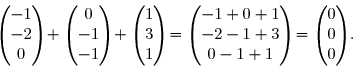
2. b) Nous devons vérifier que
De plus, nous avons :
D'où et
Nous en déduisons que le triangle OAC est rectangle et isocèle en O.
3. a) Donnons une écriture sous forme exponentielle du nombre complexe
3. b) Nous en déduisons que le triangle ABC est rectangle et isocèle en B.
4. Nous devons montrer que les points A , B , C et O appartiennent à un même cercle.
Nous savons que dans un triangle rectangle, le milieu de l'hypoténuse est le centre du cercle circonscrit à ce triangle.
Dès lors,
Le triangle OAC étant rectangle en O, le milieu de l'hypoténuse [AC] est le centre du cercle circonscrit à ce triangle.
Le rayon de ce cercle est
Le triangle ABC étant rectangle en B, le milieu de l'hypoténuse [AC] est le centre du cercle circonscrit à ce triangle.
Le rayon de ce cercle est
Par conséquent , les points A , B , C et O appartiennent à un même cercle dont le centre est le milieu de l'hypoténuse [AC] et le rayon est
5,5 points
exercice 2
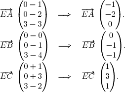
Dans l'espace rapporté à un repère orthonormal on considère les points
et le vecteur
1. Démontrons que les points A , B et C ne sont pas alignés.
Manifestement, les coordonnées des vecteurs et ne sont pas proportionnelles.
Dès lors, ces vecteurs et ne sont pas colinéaires.
Nous en déduisons que les points A , B et C ne sont pas alignés et déterminent donc un plan..
2. a) Démontrons que est un vecteur normal au plan
Puisque le vecteur est orthogonal aux vecteurs non colinéaires et nous avons montré que est un vecteur normal au plan
2. b) Nous devons déterminer une équation cartésienne du plan
Le vecteur est un vecteur normal au plan
D'où l'équation du plan est de la forme où est un nombre réel.
Nous savons que appartient à ce plan.
Donc soit
Par conséquent, une équation cartésienne du plan est
2. c) Nous devons déterminer une représentation paramétrique de la droite passant par le point O et orthogonale au plan (ABC).
Un vecteur directeur de la droite est le vecteur
Le point appartient à .
Donc une représentation paramétrique de la droite est :
soit
3. a) Montrons que les points A , B , C et D sont les sommets d'un tétraèdre.
Le point D (4 ; -2 ; 5) n'appartient pas au plan car ses coordonnées ne vérifient pas l'équation de
En effet,
Dès lors, les points A , B , C et D sont les sommets d'un tétraèdre.
3. b) Calculons la distance du point D au plan
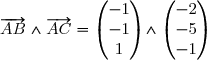
3. c) Calculons le volume du tétraèdre
Calculons
Par la question 1., nous avons : et
Nous en déduisons que
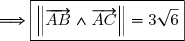
D'où
Nous savons que
Donc
Par conséquent, le volume du tétraèdre est égal à 6 unités de volume.
4. Soit la droite dont une représentation paramétrique est :
Nous devons montrer que le point appartient à la droite
Montrons qu'il existe une valeur de telle que
Par conséquent, le point appartient à la droite
De plus, la droite est perpendiculaire au plan car admet pour vecteur directeur.
5. Soit le projeté orthogonal du point sur le plan
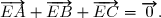
Montrons que le point est le centre de gravité du triangle
Montrons donc que
Déterminons d'abord les coordonnées du point
Par définition du point nous savons que ce point 'est le point d'intersection de la droite et du plan
Dès lors, ses coordonnées sont données en résolvant le système composé par la représentation paramétrique de et l'équation du plan
Nous en déduisons que les coordonnées de sont (0 ; 0 ; 3).
Dès lors, nous obtenons :
Or
D'où
Par conséquent, le point est le centre de gravité du triangle
10 points
probleme
Partie A (2,75 points)
On considère la fonction définie sur par
1. Nous devons calculer les limites de en et en
Calculons
Calculons
2. Nous devons étudier les variations de
La fonction est dérivable sur
Pour tout nombre réel,
Étudions le signe de sur
L'exponentielle est strictement positive sur
Dès lors le signe de est le signe de
Nous pouvons ainsi dresser le tableau de variations de
Par conséquent, la fonction est strictement croissante sur strictement décroissante sur
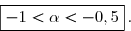
3. a) Montrons que l'équation admet une unique solution sur , notée
Sur l'intervalle la fonction g est continue et strictement croissante.
Il s'ensuit que g réalise une bijection de sur
Or
Dès lors, l'équation admet une unique solution sur
Sur l'intervalle la fonction g est continue et strictement décroissante.
Il s'ensuit que g réalise une bijection de sur
Or
Dès lors, l'équation n'admet pas de solution sur
Par conséquent, l'équation admet une unique solution sur
3. b)
D'où
4. Déterminons le signe de suivant les valeurs de
Complétons le tableau de variations de
Nous en déduisons que sur sur
Partie B (4,75 points)
On considère la fonction définie sur par et on note
sa courbe représentative dans le plan muni d'un repère orthonormé d'unité graphique 2 cm.
1. a) Nous devons calculer la limite de en
Nous en déduisons que la droite d'équation est asymptote horizontale à la courbe en -.
1. b) Nous devons calculer la limite de en
1. c) Nous devons étudier la branche infinie de en +.
Calculons
Nous en déduisons que la courbe admet une branche parabolique de direction l'axe des ordonnées en +.
2. La fonction est dérivable sur
3. Nous devons dresser le tableau de variations de
Le signe de est le signe de car l'exponentielle est toujours strictement positive.
En utilisant le résultat de la question 4. Partie A, nous obtenons :
4. Nous devons vérifier que
Par définition de , nous obtenons :
Dès lors,
5. Nous devons tracer la courbe en prenant
Partie C (2,5 points)
1. Nous devons calculer
Dès lors
Par conséquent,
2. Calculons l'aire , en cm2, de la partie du plan délimitée par la courbe
, les droites d'équations et et l'axe des abscisses.
Déterminons d'abord l'aire en unité d'aire (u.a.).
Or l'unité graphique du repère est de 2 cm.
Dès lors l'unité d'aire est 4 cm2.
Par conséquent,
Publié par malou
le
ceci n'est qu'un extrait
Pour visualiser la totalité des cours vous devez vous inscrire / connecter (GRATUIT) Inscription Gratuitese connecter
Merci à Hiphigenie / malou pour avoir contribué à l'élaboration de cette fiche
Désolé, votre version d'Internet Explorer est plus que périmée ! Merci de le mettre à jour ou de télécharger Firefox ou Google Chrome pour utiliser le site. Votre ordinateur vous remerciera !
 l'équation suivante :
 :z^2-2(1+\text i\sqrt2)z+2(-1+2\text i\sqrt2)=0.)
^2 }) sous forme algébrique.
sous forme algébrique.
^2=(\sqrt 2)^2-2\times\sqrt 2\times\text i+\text i^2 \\\overset{ { \white{ . } } } {\phantom{(\sqrt2-\text i)^2}=2-2\,\text i\sqrt 2-1} \\\overset{ { \white{ . } } } {\phantom{(\sqrt2-\text i)^2}=1-2\,\text i\sqrt 2} \\\\\Longrightarrow\quad\boxed{(\sqrt2-\text i)^2=1-2\,\text i\sqrt 2})
:z^2-2(1+\text i\sqrt2)z+2(-1+2\text i\sqrt2)=0. })

\big)^2-4\times1\times2(-1+2\,\text i\sqrt2) \\\overset{ { \white{ . } } } {\phantom{d}=4(1+2\,\text i\sqrt2-2)-8(-1+2\,\text i\sqrt2)} \\\overset{ { \white{ . } } } {\phantom{d}=4(-1+2\,\text i\sqrt2)+8-16\,\text i\sqrt2} \\\overset{ { \white{ . } } } {\phantom{d}=-4+8\,\text i\sqrt2+8-16\,\text i\sqrt2})

 \\\overset{ { \white{ . } } } {\phantom{d}=\Big(2(\sqrt2-\text i)\Big)^2\quad(\text{voir question 1. a})})
-2(\sqrt2-\text i)}{2} \\\overset{ { \white{ . } } } {\phantom{z_1}=(1+\text i\sqrt2)-(\sqrt2-\text i)} \\\overset{ { \white{ . } } } {\phantom{z_1}=1-\sqrt2+\text i\sqrt2+\text i} \\\overset{ { \white{ . } } } {\phantom{z_1}=(1-\sqrt2)+\text i(1+\sqrt2)})
+2(\sqrt2-\text i)}{2} \\\overset{ { \white{ . } } } {\phantom{z_1}=(1+\text i\sqrt2)+(\sqrt2-\text i)} \\\overset{ { \white{ . } } } {\phantom{z_1}=1+\sqrt2+\text i\sqrt2-\text i} \\\overset{ { \white{ . } } } {\phantom{z_1}=(1+\sqrt2)-\text i(1-\sqrt2)})
 }) est
est +\text i(1+\sqrt2)\;;\;(1+\sqrt2)-\text i(1-\sqrt2)\rbrace}\,.)
,}) on considère les points A , B et C d'affixes respectives :
on considère les points A , B et C d'affixes respectives : -\text i(1-\sqrt2),\;z_B=2+2\,\texti\sqrt2) et
et +\text i(1+\sqrt2).)

![\text i\,z_A=\text i\left[\overset{}{(1+\sqrt2)-\text i(1-\sqrt2)}\right] \\\overset{ { \white{ . } } } { \phantom{\text i\,z_A}=\text i\,(1+\sqrt2)+(1-\sqrt2)} \\\overset{ { \white{ . } } } { \phantom{\text i\,z_A}=z_C} \\\\\Longrightarrow\quad\boxed{z_C=\text i\,z_A}](https://latex.ilemaths.net/latex-0.tex?\text i\,z_A=\text i\left[\overset{}{(1+\sqrt2)-\text i(1-\sqrt2)}\right] \\\overset{ { \white{ . } } } { \phantom{\text i\,z_A}=\text i\,(1+\sqrt2)+(1-\sqrt2)} \\\overset{ { \white{ . } } } { \phantom{\text i\,z_A}=z_C} \\\\\Longrightarrow\quad\boxed{z_C=\text i\,z_A})
=\dfrac{\pi}{2}\end{matrix}\right.)
 et
et ![\overset{ { \white{ . } } } { \left(\overrightarrow{OA},\overrightarrow{OC}\right)=\dfrac{\pi}{2}\,[2\pi].}](https://latex.ilemaths.net/latex-0.tex?\overset{ { \white{ . } } } { \left(\overrightarrow{OA},\overrightarrow{OC}\right)=\dfrac{\pi}{2}\,[2\pi].})
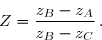
-\Big((1+\sqrt2)-\text i(1-\sqrt2)\Big)}{(2+2\,\text i\sqrt 2)-\Big((1-\sqrt2)+\text i(1+\sqrt2)\Big)} \\\overset{ { \white{ . } } } {\phantom{Z}=\dfrac{2+2\,\text i\sqrt 2-1-\sqrt2+\text i-\text i\sqrt2}{2+2\,\text i\sqrt 2-1+\sqrt2-\text i-\text i\sqrt2}} \\\overset{ { \white{ . } } } {\phantom{Z}=\dfrac{1-\sqrt 2+\text i+\text i\sqrt 2}{1+\sqrt 2-\text i+\text i\sqrt 2}} \\\overset{ { \white{ . } } } {\phantom{Z}=\dfrac{(1-\sqrt 2)+\text i\,(1+\sqrt 2)}{(1+\sqrt 2)+\text i\,(-1+\sqrt 2)}})
![\\\overset{ { \white{ . } } } {\phantom{Z}=\dfrac{\text i\,\left[\overset{}{(1+\sqrt 2)-\text i(1-\sqrt 2)}\right]}{(1+\sqrt 2)+\text i\,(-1+\sqrt 2)}} \\\overset{ { \white{ . } } } {\phantom{Z}=\dfrac{\text i\,\left[\overset{}{(1+\sqrt 2)+\text i(-1+\sqrt 2)}\right]}{(1+\sqrt 2)+\text i\,(-1+\sqrt 2)}} \\\overset{ { \white{ . } } } {\phantom{Z}=\text i} \\\overset{ { \phantom{ . } } } {\phantom{Z}=\text e^{\text i\frac{\pi}{2}}} \\\\\Longrightarrow\quad\boxed{Z=\dfrac{z_B-z_A}{z_B-z_C}=\text e^{\text i\frac{\pi}{2}}}](https://latex.ilemaths.net/latex-0.tex?\\\overset{ { \white{ . } } } {\phantom{Z}=\dfrac{\text i\,\left[\overset{}{(1+\sqrt 2)-\text i(1-\sqrt 2)}\right]}{(1+\sqrt 2)+\text i\,(-1+\sqrt 2)}} \\\overset{ { \white{ . } } } {\phantom{Z}=\dfrac{\text i\,\left[\overset{}{(1+\sqrt 2)+\text i(-1+\sqrt 2)}\right]}{(1+\sqrt 2)+\text i\,(-1+\sqrt 2)}} \\\overset{ { \white{ . } } } {\phantom{Z}=\text i} \\\overset{ { \phantom{ . } } } {\phantom{Z}=\text e^{\text i\frac{\pi}{2}}} \\\\\Longrightarrow\quad\boxed{Z=\dfrac{z_B-z_A}{z_B-z_C}=\text e^{\text i\frac{\pi}{2}}})
 Le triangle OAC étant rectangle en O , le milieu de l'hypoténuse [AC] est le centre du cercle circonscrit à ce triangle.
,}) on considère les points
on considère les points ,B(0\;;\;1\;;\;4),C(-1\;;\;-3\;;\;2),D(4\;;\;-2\;;\;5) }) et le vecteur
et le vecteur 
\\B(0\;;\;1\;;\;4)\end{matrix}\right.\quad\Longrightarrow\quad\overrightarrow {AB}\begin{pmatrix}0-1\\1-2\\4-3\end{pmatrix}\quad\Longrightarrow\quad\overrightarrow {AB}\begin{pmatrix}-1\\-1\\1\end{pmatrix} \\\\\left\lbrace\begin{matrix}A(1\;;\;2\;;\;3)\\C(-1\;;\;-3\;;\;2)\end{matrix}\right.\quad\Longrightarrow\quad\overrightarrow {AC}\begin{pmatrix}-1-1\\-3-2\\2-3\end{pmatrix}\quad\Longrightarrow\quad\overrightarrow {AC}\begin{pmatrix}-2\\-5\\-1\end{pmatrix})
 et
et  ne sont pas proportionnelles.
 est un vecteur normal au plan
 . })
\times(-1)+1\times(-1)+(-1)\times1=0 \\\phantom{WWWWW}\quad\Longrightarrow\quad\boxed{\vec n\perp\overrightarrow {AB}} \\\\\left\lbrace\begin{matrix}\vec n\begin{pmatrix}-2\\1\\-1\end{pmatrix}\\\overset{ { \white{ . } } } {\overrightarrow {AC}\begin{pmatrix}-2\\-5\\-1\end{pmatrix} } \end{matrix}\right.\quad\Longrightarrow\quad\vec n\cdot\overrightarrow {AC}=(-2)\times(-2)+1\times(-5)+(-1)\times(-1)=0 \\\phantom{WWWWW}\quad\Longrightarrow\quad\boxed{\vec n\perp\overrightarrow {AC}})
 nous avons montré que
  est un vecteur normal au plan
  }) est de la forme
est de la forme  où
où  est un nombre réel.
 }) appartient à ce plan.
appartient à ce plan. soit
soit 
}) passant par le point O et orthogonale au plan (ABC).
passant par le point O et orthogonale au plan (ABC). 
}) appartient à
appartient à }}\times k\\y={\blue{0}}+{\red{1}}\times k\phantom{xxx}\\z={\blue{0}}+{\red{(-1)}}\times k\end{matrix}\right.\quad \quad(k\in\R) })
:\left\lbrace\begin{matrix}x=-2k\\y=k\phantom{xx}\\z=-k\end{matrix}\right.\quad \quad(k\in\R)} })

) }) du point D au plan
du point D au plan )=\dfrac{\mid -2\times4+(-2)-5+3\mid}{\sqrt{(-2)^2+1^2+(-1)^2}} \\\overset{ { \white{ . } } } {{ \phantom{ d(D,(ABC))}=\dfrac{\mid -12\mid}{\sqrt{6}}=\dfrac{12}{\sqrt{6}}=\dfrac{12\sqrt 6}{\sqrt{6}\sqrt6}=\dfrac{12\sqrt 6}{6}=2\sqrt6}} \\\\\overset{ { \white{ . } } } { \Longrightarrow\boxed{ d(D,(ABC))=2\sqrt6}\,.})
 du tétraèdre
))

 et
et 

\times(-1)-1\times(-5)\\1\times(-2)-(-1)\times(-1)\\ (-1)\times(-5)-(-1)\times(-2)\end{pmatrix}} \\\overset{ { \white{ . } } } {\phantom{WWWW}=\begin{pmatrix}6\\-3\\3\end{pmatrix}})
^2+3^2}=\sqrt{54}=3\sqrt{6}})
)=2\sqrt6}\,.})
) =\dfrac16\times3\sqrt6\times 2\sqrt6 =6. })
 est égal à 6 unités de volume.
 }) la droite dont une représentation paramétrique est :
la droite dont une représentation paramétrique est : } )
 appartient à la droite
 . })
 telle que
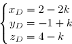

 pour vecteur directeur.
  le projeté orthogonal du point
  sur le plan
 .})
 est le centre de gravité du triangle

 nous savons que ce point
 { }) et du plan
et du plan  }) et l'équation du plan
et l'équation du plan +(-1+k)-(4-k)+3=0\end{matrix}\right. } \\\overset{ { \white{ . } } } {\phantom{WWWWWWWWW}\quad\Longleftrightarrow\quad \left\lbrace\begin{matrix}x=2-2k\phantom{}\\y=-1+k\\z=4-k\phantom{v}\\-6+6k=0\end{matrix}\right. } \\\overset{ { \white{ . } } } {\phantom{WWWWWWWWW}\quad\Longleftrightarrow\quad \left\lbrace\begin{matrix}x=2-2k\phantom{}\\y=-1+k\\z=4-k\phantom{v}\\k=1\phantom{xxxx}\end{matrix}\right. })


 est le centre de gravité du triangle
 définie sur
  par
par =2+x\,\text e^{-x}.})
 et en
et en 
 Calculons
 .})
=-\infty .\\\overset{ { \white{ . } } } {\phantom{WWWWWWWWxWW}\quad\Longrightarrow\quad\boxed{\lim\limits_{x\to-\infty}g(x)=-\infty}})
.})
 \\\phantom{WWWWWWWwWW}\quad\Longrightarrow\quad\lim\limits_{x\to+\infty}(2+x\,\text e^{-x})=2 .\\\overset{ { \white{ . } } } {\phantom{WWWWWWWxWW}\quad\Longrightarrow\quad\boxed{\lim\limits_{x\to+\infty}g(x)=2}})


 réel,
réel, =(2+x\,\text e^{-x})' \\\overset{ { \white{ . } } } {\phantom{g'(x)}=0+(x\,\text e^{-x})' } \\\overset{ { \white{ . } } } {\phantom{g'(x)}=x'\times\text e^{-x}+x\times(\text e^{-x})' } \\\overset{ { \white{ . } } } {\phantom{g'(x)}=1\times\text e^{-x}+x\times(-\,\text e^{-x}) } \\\overset{ { \phantom{ . } } } {\phantom{g'(x)}=\text e^{-x}-x\,\text e^{-x} } \\\overset{ { \phantom{ . } } } {\phantom{g'(x)}=(1-x)\,\text e^{-x} } \\\\\Longrightarrow\quad\boxed{g'(x)=(1-x)\,\text e^{-x} })
 }) sur
sur }) est le signe de
est le signe de .})
&&+&+&0&-&-&\\&&&&&&&\\\hline \end{array} )

&&+&+&0&-&-&\\&&&&&&&\\\hline&&&&2+\text e^{-1}\approx2,37&&&\\g(x)&&\nearrow&\nearrow&&\searrow&\searrow&\\&-\infty&&&&&&2\\\hline \end{array} )
 est strictement croissante sur
 ![\overset{ { \white{ . } } } { ]-\infty\;;\;1[ }](https://latex.ilemaths.net/latex-0.tex?\overset{ { \white{ . } } } { ]-\infty\;;\;1[ })
 strictement décroissante sur
 ![\overset{ { \white{ . } } } { ]1\;;\;+\infty[. }](https://latex.ilemaths.net/latex-0.tex?\overset{ { \white{ . } } } { ]1\;;\;+\infty[. })
=0}) admet une unique solution sur
admet une unique solution sur  , notée
![\overset{ { \white{ . } } } { ]-\infty\;;\;1[, }](https://latex.ilemaths.net/latex-0.tex?\overset{ { \white{ . } } } { ]-\infty\;;\;1[, }) la fonction g est continue et strictement croissante.
la fonction g est continue et strictement croissante.![\overset{ { \white{ . } } } { ]-\infty\;;\;1[}](https://latex.ilemaths.net/latex-0.tex?\overset{ { \white{ . } } } { ]-\infty\;;\;1[}) sur
sur ![\overset{ { \white{ . } } } { g( ]-\infty\;;\;1[)=]-\infty\;;\;2+\text e^{-1}[.}](https://latex.ilemaths.net/latex-0.tex?\overset{ { \white{ . } } } { g( ]-\infty\;;\;1[)=]-\infty\;;\;2+\text e^{-1}[.})
![\overset{ { \white{ . } } } {0\in\,]-\infty\;;\;2+\text e^{-1}[. }](https://latex.ilemaths.net/latex-0.tex?\overset{ { \white{ . } } } {0\in\,]-\infty\;;\;2+\text e^{-1}[. })
 sur
sur ![\overset{ { \white{ . } } }{ ]-\infty\;;\;1[.}](https://latex.ilemaths.net/latex-0.tex?\overset{ { \white{ . } } }{ ]-\infty\;;\;1[.})
![\overset{ { \white{ . } } } { ]1\;;\;+\infty[, }](https://latex.ilemaths.net/latex-0.tex?\overset{ { \white{ . } } } { ]1\;;\;+\infty[, }) la fonction g est continue et strictement décroissante.
la fonction g est continue et strictement décroissante.![\overset{ { \white{ . } } } { ]1\;;\;+\infty[}](https://latex.ilemaths.net/latex-0.tex?\overset{ { \white{ . } } } { ]1\;;\;+\infty[}) sur
sur ![\overset{ { \white{ . } } } { g( ]1\;;\;+\infty[)=]2\;;\;2+\text e^{-1}[.}](https://latex.ilemaths.net/latex-0.tex?\overset{ { \white{ . } } } { g( ]1\;;\;+\infty[)=]2\;;\;2+\text e^{-1}[.})
![\overset{ { \white{ . } } } {0\notin\,]2\;;\;2+\text e^{-1}[. }](https://latex.ilemaths.net/latex-0.tex?\overset{ { \white{ . } } } {0\notin\,]2\;;\;2+\text e^{-1}[. })
![\overset{ { \white{ . } } }{ ]1\;;\;+\infty[.}](https://latex.ilemaths.net/latex-0.tex?\overset{ { \white{ . } } }{ ]1\;;\;+\infty[.})

=2-\text e\approx-0,718<0\\\overset{ { \white{ . } } } {g(-0,5)\approx1,176>0\phantom{xxxxx}}\end{matrix}\right.\quad\Longrightarrow\quad g(-1)\times g(-0,5)<0)
}) suivant les valeurs de
suivant les valeurs de 
&&\nearrow&0&\nearrow&&\searrow&\\&-\infty&&&&&&2\\\hline \end{array} )
<0 }) sur
sur ![\overset{ { \white{ . } } } { ]-\infty\;;\;\alpha[ }](https://latex.ilemaths.net/latex-0.tex?\overset{ { \white{ . } } } { ]-\infty\;;\;\alpha[ })

>0 }) sur
sur ![\overset{ { \white{ . } } } { ]\alpha\;;\;+\infty[. }](https://latex.ilemaths.net/latex-0.tex?\overset{ { \white{ . } } } { ]\alpha\;;\;+\infty[. })
 définie sur
 =1+\text e^{2x}+(x-1)\,\text e^x}) et on note
et on note
}) sa courbe représentative dans le plan muni d'un repère orthonormé
sa courbe représentative dans le plan muni d'un repère orthonormé }) d'unité graphique 2 cm.
d'unité graphique 2 cm.
=-\infty} \\\overset{ { \white{ . } } } {\lim\limits_{x\to-\infty}\text e^{x}=0\phantom{WWW}}\end{matrix}\right.\quad\Longrightarrow\quad\left\lbrace\begin{matrix}\lim\limits_{x\to-\infty}\text e^{2x}=0\phantom{WWWWWWWWWWWWW} \\\overset{ { \phantom{ . } } } {\lim\limits_{x\to-\infty}(x-1)\,\text e^x=0\quad(\text{croissances comparées})}\end{matrix}\right. \\\phantom{WWWWWWWwWW}\quad\Longrightarrow\quad\lim\limits_{x\to-\infty}\Big(1+\text e^{2x}+(x-1)\,\text e^x\Big)=1+0+0\\\overset{ { \white{ . } } } {\phantom{WWWWWWWxWW}\quad\Longrightarrow\quad\boxed{\lim\limits_{x\to-\infty}f(x)=1}})
 est asymptote horizontale à la courbe
  .
.=+\infty} \\\overset{ { \white{ . } } } {\lim\limits_{x\to+\infty}\text e^{x}=+\infty\phantom{WW}}\end{matrix}\right.\quad\Longrightarrow\quad\left\lbrace\begin{matrix}\lim\limits_{x\to+\infty}\text e^{2x}=+\infty\phantom{WW} \\\overset{ { \phantom{ . } } } {\lim\limits_{x\to+\infty}(x-1)\,\text e^x=+\infty}\end{matrix}\right.\\\phantom{WWWWWWWwWW}\quad\Longrightarrow\quad\lim\limits_{x\to+\infty}\Big(1+\text e^{2x}+(x-1)\,\text e^x\Big)=+\infty \\\overset{ { \white{ . } } } {\phantom{WWWWWWWxWW}\quad\Longrightarrow\quad\boxed{\lim\limits_{x\to+\infty}f(x)=+\infty}})
}{x}\,. })
}{x}=\dfrac{1+\text e^{2x}+(x-1)\,\text e^x}{x} \\\overset{ { \white{ . } } } {\Longrightarrow\quad \boxed{\forall\,x\neq0,\quad \dfrac{f(x)}{x}=\dfrac{1}{x}+\dfrac{\text e^{2x}}{x}+\left(1-\dfrac{1}{x}\right)\,\text e^x}})
![\text{Or }\;\left\lbrace\begin{matrix}\lim\limits_{x\to+\infty}\dfrac{1}{x}=0\phantom{WWWWWWWWWWW}\\\overset{ { \white{ . } } } {\lim\limits_{x\to+\infty}\dfrac{\text e^{2x}}{x}=0 \quad(\text{croissances comparées})}\\\overset{ { \white{ . } } } {\lim\limits_{x\to+\infty}\left(1-\dfrac{1}{x}\right)=1-0=1\phantom{WWWWW}}\\\overset{ { \white{ . } } } {\lim\limits_{x\to+\infty}\text e^x=+\infty\phantom{WWWWWWWWWW}}\end{matrix}\right. \\\\\quad\Longrightarrow\quad\lim\limits_{x\to+\infty}\left[\dfrac{1}{x}+\dfrac{\text e^{2x}}{x}+\left(1-\dfrac{1}{x}\right)\,\text e^x\right]=+\infty \\\\\quad\Longrightarrow\quad\boxed{\lim\limits_{x\to+\infty}\dfrac{f(x)}{x}=+\infty}](https://latex.ilemaths.net/latex-0.tex?\text{Or }\;\left\lbrace\begin{matrix}\lim\limits_{x\to+\infty}\dfrac{1}{x}=0\phantom{WWWWWWWWWWW}\\\overset{ { \white{ . } } } {\lim\limits_{x\to+\infty}\dfrac{\text e^{2x}}{x}=0 \quad(\text{croissances comparées})}\\\overset{ { \white{ . } } } {\lim\limits_{x\to+\infty}\left(1-\dfrac{1}{x}\right)=1-0=1\phantom{WWWWW}}\\\overset{ { \white{ . } } } {\lim\limits_{x\to+\infty}\text e^x=+\infty\phantom{WWWWWWWWWW}}\end{matrix}\right. \\\\\quad\Longrightarrow\quad\lim\limits_{x\to+\infty}\left[\dfrac{1}{x}+\dfrac{\text e^{2x}}{x}+\left(1-\dfrac{1}{x}\right)\,\text e^x\right]=+\infty \\\\\quad\Longrightarrow\quad\boxed{\lim\limits_{x\to+\infty}\dfrac{f(x)}{x}=+\infty})
=\Big(1+\text e^{2x}+(x-1)\,\text e^x\Big)' \\\overset{ { \white{ . } } } { \phantom{f'(x)}=0+(2x)'\,\text e^{2x}+(x-1)'\times\text e^x+(x-1)\times(\text e^x)' } \\\overset{ { \white{ . } } } { \phantom{f'(x)}=2\,\text e^{2x}+1\times\text e^x+(x-1)\times\text e^x } \\\overset{ { \white{ . } } } { \phantom{f'(x)}=2\,\text e^{2x}+\text e^x+x\,\text e^x -\text e^x })
}=2\,\text e^{2x}+x\,\text e^x } \\\overset{ { \white{ . } } } { \phantom{f'(x)}=2\,\text e^{2x}+x\,\text e^{-x}\text e^{2x} } \\\overset{ { \white{ . } } } { \phantom{f'(x)}=(2+x\,\text e^{-x})\,\text e^{2x} } \\\overset{ { \phantom{ . } } } { \phantom{f'(x)}=g(x)\,\text e^{2x} } \\\\\Longrightarrow\quad\boxed{\forall\,x\in\R,\;f'(x)=g(x)\,\text e^{2x}})

}) est le signe de
est le signe de }) car l'exponentielle est toujours strictement positive.
car l'exponentielle est toujours strictement positive.&&-&0&+&&\\&&&&&&\\\hline&&&&&&\\f'(x)&&-&0&+&&\\&&&&&&\\\hline&1&&&&+\infty&\\f(x)&&\searrow&&\nearrow&&\\&&&f(\alpha)&&&\\\hline \end{array} )
=\dfrac{-\alpha ^2+2\alpha +4}{4}.})
 , nous obtenons :
=0\quad\Longleftrightarrow\quad 2+\alpha\,\text e^{-\alpha}=0 \\\overset{ { \white{ . } } } {\phantom{g(\alpha)=0}\quad\Longleftrightarrow\quad \alpha\,\text e^{-\alpha}=-2} \\\overset{ { \white{ . } } } {\phantom{g(\alpha)=0}\quad\Longleftrightarrow\quad \text e^{-\alpha}=-\dfrac{2}{\alpha}} \\\overset{ { \white{ . } } } {\phantom{g(\alpha)=0}\quad\Longleftrightarrow\quad \boxed{\text e^{\alpha}=-\dfrac{\alpha}{2}}})
=1+\text e^{2\alpha}+(\alpha-1)\,\text e^\alpha \\\overset{ { \white{ . } } } {\phantom{f(\alpha)}=1+(\text e^{\alpha})^2+(\alpha-1)\,\text e^\alpha} \\\overset{ { \white{ . } } } {\phantom{f(\alpha)}=1+\left(-\dfrac{\alpha}{2}\right)^2+(\alpha-1)\,\left(-\dfrac{\alpha}{2}\right)} \\\overset{ { \white{ . } } } {\phantom{f(\alpha)}=1+\dfrac{\alpha^2}{4}+(\alpha-1)\,\left(-\dfrac{\alpha}{2}\right)})
}=1+\dfrac{\alpha^2}{4}-\dfrac{\alpha^2}{2}+\dfrac{\alpha}{2}} \\\overset{ { \white{ . } } } {\phantom{f(\alpha)}=\dfrac44+\dfrac{\alpha^2}{4}-\dfrac{2\alpha^2}{4}+\dfrac{2\alpha}{4}} \\\overset{ { \white{ . } } } {\phantom{f(\alpha)}=\dfrac{-\alpha^2+2\alpha+4}{4}} \\\\\Longrightarrow\quad\boxed{f(\alpha)=\dfrac{-\alpha^2+2\alpha+4}{4}})
}) en prenant
en prenant 
\,\text e^x\,\text{d}x.})
![\underline{\text{Formule de l'intégrale par parties}}\ :\ {\blue{\displaystyle\int_0^{1}u(x)v'(x)\,\text{d}x=\left[\overset{}{u(x)v(x)}\right]\limits_0^1- \displaystyle\int\limits_0^1u'(x)v(x)\,\text{d}x}}. \\ \\ \left\lbrace\begin{matrix}u(x)=x-1\quad\Longrightarrow\quad u'(x)=1 \\\\v'(x)=\text e^x\phantom{W}\quad\Longrightarrow\quad v(x)=\text e^x\end{matrix}\right.](https://latex.ilemaths.net/latex-0.tex?\underline{\text{Formule de l'intégrale par parties}}\ :\ {\blue{\displaystyle\int_0^{1}u(x)v'(x)\,\text{d}x=\left[\overset{}{u(x)v(x)}\right]\limits_0^1- \displaystyle\int\limits_0^1u'(x)v(x)\,\text{d}x}}. \\ \\ \left\lbrace\begin{matrix}u(x)=x-1\quad\Longrightarrow\quad u'(x)=1 \\\\v'(x)=\text e^x\phantom{W}\quad\Longrightarrow\quad v(x)=\text e^x\end{matrix}\right. )
![\overset{ { \white{ . } } } { I=\left[\overset{}{(x-1)\,\text e^x}\right]_0^1-\displaystyle\int_0^{1}1\times\text{e}^x\,\text{d}x=\left[\overset{}{(x-1)\,\text e^x}\right]_0^1-\displaystyle\int_0^{1}\text{e}^x\,\text{d}x}](https://latex.ilemaths.net/latex-0.tex?\overset{ { \white{ . } } } { I=\left[\overset{}{(x-1)\,\text e^x}\right]_0^1-\displaystyle\int_0^{1}1\times\text{e}^x\,\text{d}x=\left[\overset{}{(x-1)\,\text e^x}\right]_0^1-\displaystyle\int_0^{1}\text{e}^x\,\text{d}x} )

![\\\\\phantom{I}=\left[\overset{}{(x-1)\,\text e^x}\right]_0^1-\left[\overset{}{\text e^x}\right]_0^1 \\\overset{ { \white{ . } } } { \phantom{I}=[0-(-\text e^0)]-(\text e^1-\text e^0)} \\\overset{ { \white{ . } } } { \phantom{I}=1-\text e+1} \\\overset{ { \phantom{ . } } } { \phantom{I}=2-\text e}](https://latex.ilemaths.net/latex-0.tex?\\\\\phantom{I}=\left[\overset{}{(x-1)\,\text e^x}\right]_0^1-\left[\overset{}{\text e^x}\right]_0^1 \\\overset{ { \white{ . } } } { \phantom{I}=[0-(-\text e^0)]-(\text e^1-\text e^0)} \\\overset{ { \white{ . } } } { \phantom{I}=1-\text e+1} \\\overset{ { \phantom{ . } } } { \phantom{I}=2-\text e})

 , en cm2, de la partie du plan délimitée par la courbe
 } } } { (\mathscr{C}) }) , les droites d'équations
, les droites d'équations  et
et  et l'axe des abscisses.
 en unité d'aire (u.a.).
![\mathscr{A}=\displaystyle\int_{0}^{1} f(x)\,\text{d}x\;(\text{u.a.}) \\\overset{ { \white{ . } } } { \phantom{A}=\displaystyle\int_{0}^{1} \Big(1+\text e^{2x}+(x-1)\,\text e^x\Big)\,\text{d}x\;(\text{u.a.})} \\\overset{ { \white{ . } } } { \phantom{A}=\displaystyle\int_{0}^{1} \Big(1+\text e^{2x}\Big)\,\text{d}x+\displaystyle\int_{0}^{1}(x-1)\,\text e^x\,\text{d}x\;(\text{u.a.})} \\\overset{ { \white{ . } } } { \phantom{A}=\left[x+\dfrac{\text e^{2x}}{2}\right]_0^1+(2-\text e)\;(\text{u.a.})} \\\overset{ { \white{ . } } } { \phantom{A}=(1+\dfrac{\text e^2}{2})-(0+\dfrac12)+(2-\text e)\;(\text{u.a.})} \\\overset{ { \white{ . } } } { \phantom{A}=\dfrac12+\dfrac{\text e^2}{2}+2-\text e\;(\text{u.a.})}](https://latex.ilemaths.net/latex-0.tex?\mathscr{A}=\displaystyle\int_{0}^{1} f(x)\,\text{d}x\;(\text{u.a.}) \\\overset{ { \white{ . } } } { \phantom{A}=\displaystyle\int_{0}^{1} \Big(1+\text e^{2x}+(x-1)\,\text e^x\Big)\,\text{d}x\;(\text{u.a.})} \\\overset{ { \white{ . } } } { \phantom{A}=\displaystyle\int_{0}^{1} \Big(1+\text e^{2x}\Big)\,\text{d}x+\displaystyle\int_{0}^{1}(x-1)\,\text e^x\,\text{d}x\;(\text{u.a.})} \\\overset{ { \white{ . } } } { \phantom{A}=\left[x+\dfrac{\text e^{2x}}{2}\right]_0^1+(2-\text e)\;(\text{u.a.})} \\\overset{ { \white{ . } } } { \phantom{A}=(1+\dfrac{\text e^2}{2})-(0+\dfrac12)+(2-\text e)\;(\text{u.a.})} \\\overset{ { \white{ . } } } { \phantom{A}=\dfrac12+\dfrac{\text e^2}{2}+2-\text e\;(\text{u.a.})} )
} \\\\\Longrightarrow\quad\boxed{\mathscr{A}=\dfrac{\text e^2}{2}-\text e+\dfrac52\,\;(\text{u.a.})})
\text{cm}^2\quad\Longrightarrow\quad\boxed{\mathscr{A}=\left(2\,\text e^2-4\,\text e+10\right)\text{cm}^2})
 Voir la correction
 forum de terminale