Fiche de mathématiques

Télécharger (GRATUIT)

Ile mathématiques > maths bac > Bac 2024

Bac Général Spécialité Mathématiques

Centres étrangers Jour 1

5 points

exercice 1

Bac général spécialité maths 2024 Centres étrangers Jour 1 : image 2

Bac général spécialité maths 2024 Centres étrangers Jour 1 : image 6

4 points

exercice 2

Bac général spécialité maths 2024 Centres étrangers Jour 1 : image 7

Bac général spécialité maths 2024 Centres étrangers Jour 1 : image 8

5 points

exercice 3

Bac général spécialité maths 2024 Centres étrangers Jour 1 : image 5

Bac général spécialité maths 2024 Centres étrangers Jour 1 : image 3

6 points

exercice 4

Bac général spécialité maths 2024 Centres étrangers Jour 1 : image 1

Voir la correction

Bac général spécialité maths 2024 Centres étrangers Jour 1

5 points

exercice 1

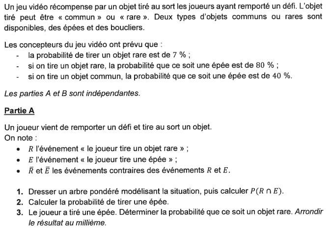
Un jeu vidéo récompense par un objet tiré au sort les joueurs ayant remporté un défi.

$\overset{ { \white{ . } } }{\bullet}{\white{x}}$ La probabilité de tirer un objet rare est de 7 %.
$\overset{ { \white{ . } } }{\bullet}{\white{x}}$ Si on tire un objet rare, la probabilité que ce soit une épée est de 80 %.
$\overset{ { \white{ . } } }{\bullet}{\white{x}}$ Si on tire un objet commun, la probabilité que ce soit une épée est de 40 %.

Partie A

Un joueur vient de remporter un défi et tire au sort un objet.

1. Dressons un arbre pondéré modélisant la situation, puis calculons $\overset{ { \white{ . } } } {P(R\cap E). }$

Bac général spécialité maths 2024 Centres étrangers Jour 1 : image 13

${ \white{ xxi } }$ $P(R\cap E)=P(R)\times P_R(E) \\\overset{ { \phantom{ . } } } { \phantom{P(R\cap E)}=0,07\times0,8} \\\overset{ { \phantom{ . } } } { \phantom{P(R\cap E)}=0,056} \\\\\Longrightarrow\quad\boxed{P(R\cap E)=0,056}$

2. Nous devons calculer $\overset{ { \white{ . } } } { P(E) }$

Les événements $\overset{{\white{_.}}}{R}$ et $\overline{R}$ forment une partition de l'univers.
En utilisant la formule des probabilités totales, nous obtenons :

${ \white{ xxi } }$ $P(E)=P(R\cap E)+P(\overline{R}\cap E) \\\overset{ { \white{ . } } } {\phantom{P(E)}=0,056+P(\overline R)\times P_{\overline R}(E)} \\\overset{ { \white{ . } } } {\phantom{P(E)}=0,056+0,93\times0,4} \\\overset{ { \white{ . } } } {\phantom{P(E)}=0,428} \\\\\Longrightarrow\quad\boxed{P(E)=0,428}$

Par conséquent, la probabilité de tirer une épée est égale à 0,428.

3. Le joueur a tiré une épée.
Déterminons la probabilité que ce soit un objet rare.

Nous devons déterminer $\overset{{\white{.}}}{P_E(R).}$

${ \white{ xxi } }$ $P_E(R)=\dfrac{P(R\cap E)}{P(E)}=\dfrac{0,056}{0,428}\approx0,131 \\\\\Longrightarrow\quad\boxed{P_E(R)\approx0,131}$

D'où, sachant que le joueur a tiré une épée, la probabilité que ce soit un objet rare est environ égale à 0,131.

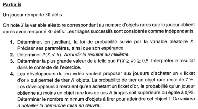
Partie B

Un joueur remporte 30 défis.

On note $\overset{ { \white{ _. } } } { X }$ la variable aléatoire correspondant au nombre d'objets rares que le joueur obtient après avoir remporté 30 défis.
Les tirages successifs sont considérés comme indépendants.

1. Lors de cette expérience, on répète 30 fois des épreuves identiques et indépendantes.
Chaque épreuve comporte deux issues :
Succès : '' l'objet tiré est rare'' dont la probabilité est $\overset{ { \white{ . } } } { p=0,07 }$
Echec : '' l'objet tiré n'est pas rare'' dont la probabilité est $\overset{ { \white{ . } } } {1-p=1-0,07=0,93. }$
La variable aléatoire $\overset{ { \white{ _. } } } { X }$ compte le nombre d'objets rares tirés à l'issue des 30 défis, soit le nombre de succès à la fin de la répétition des épreuves.
D'où la variable aléatoire $\overset{ { \white{ _. } } } { X }$ suit une loi binomiale $\overset{ { \white{ . } } }{ \mathscr{ B }(30\,;\,0,07) }$ .
Cette loi est donnée par :

$\boxed{ P(X=k)=\begin{pmatrix}30\\k\end{pmatrix}\times0,07^k\times0,93^{ 30-k } }$

2. Nous devons déterminer $\overset{ { \white{ . } } } {P(X<6). }$

$P(X<6)=P(X\le 5) \\\overset{ { \phantom{ . } } } { \phantom{P(X<6)}=P(X=0)+P(X=1)+P(X=2)+P(X=3)+P(X=4)+P(X=5)} \\\overset{ { \phantom{ . } } } { \phantom{P(X<6)}=\begin{pmatrix}30\\0\end{pmatrix}\times0,07^0\times0,93^{ 30 }+\begin{pmatrix}30\\1\end{pmatrix}\times0,07^1\times0,93^{ 29 }+\cdots+\begin{pmatrix}30\\5\end{pmatrix}\times0,07^5\times0,93^{ 25 }}$

À l'aide d'une calculatrice, nous obtenons : $\overset{ { \white{ . } } } { \boxed{P(X<0,6)\approx 0,984}\,. }$

3. Nous devons déterminer la plus grande valeur de $\overset{ { \white{ _. } } } { k }$ telle que $\overset{ { \white{ . } } } { P(X\ge k)\ge 0,5. }$

À l'aide d'une calculatrice, nous obtenons :

${ \white{ xxi } }$ $\overset{ { \white{ . } } }{\bullet}{\white{x}}P(X\ge0)=1\;{\red{\ge0,5}} \\\\\overset{ { \phantom{ . } } }{\bullet}{\phantom{x}}P(X\ge1)=1-P(X=0)=1-0,113=0,887\;{\red{\ge0,5}} \\\\\overset{ { \phantom{ . } } }{\bullet}{\phantom{x}}P(X\ge2)=1-P(X\le1)=1-0,369=0,631\;{\red{\ge0,5}} \\\\\overset{ { \phantom{ . } } }{\bullet}{\phantom{x}}P(X\ge3)=1-P(X\le2)=1-0,649=0,351\;{\red{<0,5}}$

Par conséquent, la plus grande valeur de $\overset{ { \white{ _. } } } { k }$ telle que $\overset{ { \white{ . } } } { P(X\ge k)\ge 0,5 }$ est $\overset{ { \white{ . } } } {\boxed{k=2}\,. }$

Dans le contexte de l'exercice, cela signifie que la probabilité qu'un joueur tire au moins 2 objets rares est supérieure à 0,5.

4. Nous devons déterminer le nombre $\overset{ { \white{ _. } } } { N }$ de tirages à effectuer pour que la probabilité de tirer au moins un objet rare soit supérieure ou égale à 0,95.

On note $\overset{ { \white{ _. } } } { Y }$ la variable aléatoire correspondant au nombre d'objets rares que le joueur obtient après avoir remporté $\overset{ { \white{ . } } } { N }$ défis.
La variable aléatoire $\overset{ { \white{ _. } } } { Y }$ suit une loi binomiale $\overset{ { \white{ . } } }{ \mathscr{ B }(N\,;\,0,07) }$ .
Nous devons déterminer le plus petit entier $\overset{ { \white{ _. } } } { N }$ tel que $\overset{ { \white{ . } } } { P(Y\ge1)\ge0,95. }$

Nous obtenons :

$P(Y\ge1)\ge0,95\quad\Longleftrightarrow\quad 1-P(Y=0)\ge0,95 \\ \overset{ { \phantom{ . } } } { \phantom{P(Y\ge1)\ge0,95}\quad\Longleftrightarrow\quad 1-0,95\ge P(Y=0)} \\ \overset{ { \phantom{ . } } } { \phantom{P(Y\ge1)\ge0,95}\quad\Longleftrightarrow\quad P(Y=0)\le0,05} \\ \overset{ { \phantom{ . } } } { \phantom{P(Y\ge1)\ge0,95}\quad\Longleftrightarrow\quad \begin{pmatrix}N\\0\end{pmatrix}\times0,07^0\times0,93^{ N }\le0,05} \\ \overset{ { \phantom{ . } } } { \phantom{P(Y\ge1)\ge0,95}\quad\Longleftrightarrow\quad 0,93^{ N }\le0,05}$

$\\ \overset{ { \phantom{ . } } } { \phantom{P(Y\ge1)\ge0,95}\quad\Longleftrightarrow\quad \ln0,93^{ N }\le\ln0,05} \\ \overset{ { \phantom{ . } } } { \phantom{P(Y\ge1)\ge0,95}\quad\Longleftrightarrow\quad N\ln0,93\le\ln0,05} \\ \overset{ { \phantom{ . } } } { \phantom{P(Y\ge1)\ge0,95}\quad\Longleftrightarrow\quad N\ge\dfrac{\ln0,05}{\ln0,93}\quad(\text{changement de sens de l'inégalité car }\ln0,93<0)} \\\\\text{Or }\dfrac{\ln0,05}{\ln0,93}\approx41,28$

Le plus petit nombre entier $\overset{ { \white{ _. } } } { N }$ vérifiant l'inégalité est 42.

Par conséquent, le joueur doit effectuer au moins 42 tirages pour que la probabilité de tirer au moins un objet rare soit supérieure ou égale à 0,95.

4 points

exercice 2

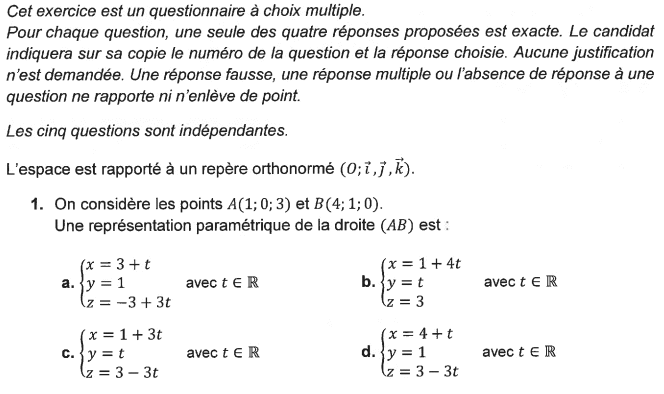
L'espace est rapporté à un repère orthonormé $(O;\vec i,\vec j,\vec k).$

Énoncé n°1 : Réponse c.

On considère les points $\overset{ { \white{ . } } } { A(1;0;3)} }$ et $\overset{ { \white{ . } } } { B(4;1;0).} }$
Une représentation paramétrique de la droite $\overset{ { \white{ . } } } { (AB)} }$ est : $\overset{ { \white{ . } } } { {\red{\left\lbrace\begin{matrix}x=1+3t\\y=t\phantom{xxxx}\\z=3-3t\end{matrix}\right.\quad\text{avec }t\in\R.}} }$

Déterminons une représentation paramétrique de la droite $\overset{ { \white{ . } } } { (AB). }$

Un vecteur directeur de $\overset{ { \white{ . } } } { (AB) }$   est le vecteur $\overset{ { \white{ . } } } { \overrightarrow{AB}\,\begin{pmatrix}4-1\\ 1-0\\0-3\end{pmatrix}\quad\Longrightarrow\quad \overrightarrow{AB}\,\begin{pmatrix}{\red{3}}\\ {\red{1}}\\ {\red{-3}}\end{pmatrix} }$
Le point $\overset{ { \white{ . } } } { A\,({\blue{1}}\;;\;{\blue{0}}\;;\;{\blue{3}}) }$ appartient à la droite $\overset{ { \white{ . } } } { (AB). }$

D'où, une représentation paramétrique de la droite $\overset{ { \white{ . } } } { (AB)}$ est : $\overset{ { \white{ . } } } {\left\lbrace\begin{matrix}x={\blue{1}}+{\red{3}}\times t\phantom{XX}\\\overset{ { \phantom{ . } } } {y={\blue{0}}+{\red{1}}\times t}\phantom{XX}\\z={\blue{3}}+{\red{(-3)}}\times t\end{matrix}\right.\quad \quad(t\in\R) }$
soit $\overset{ { \phantom{ . } } } { \boxed{(AB):\left\lbrace\begin{matrix}x=1+3t\\\overset{ { \white{ . } } } {y=t\phantom{xxxx}}\\z=3-3t\end{matrix}\right.\quad \quad (t\in\R)} }$

La proposition c. est donc correcte.

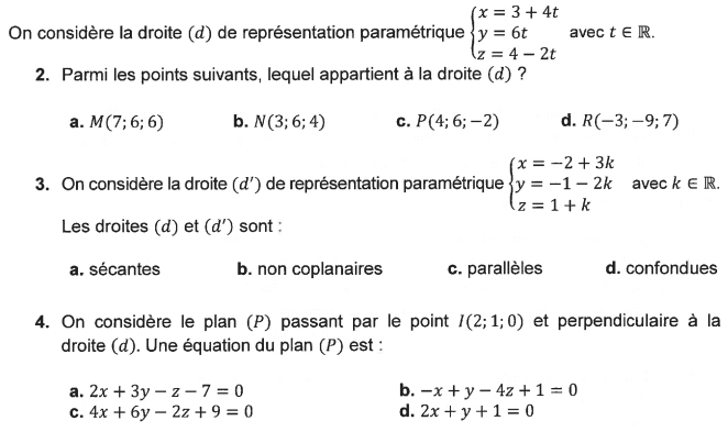
On considère la droite $\overset{ { \white{ . } } } { (d) }$ de représentation paramétrique $\overset{ { \white{ . } } } {\left\lbrace\begin{matrix}x=3+4t\\\overset{ { \white{ . } } } {y=6t\phantom{xxx}}\\z=4-2t\end{matrix}\right.\quad \quad \text{avec } t\in\R. }$

Énoncé n°2 : Réponse d.

Le point $\overset{ { \white{ . } } } {{\red{ R(-3;-9;7)}}} }$ appartient à la droite $\overset{ { \white{ . } } } { (d).} }$

Vérifions qu'il existe une valeur de $\overset{ { \white{ . } } } { t }$ vérifiant le système suivant :    $\overset{ { \white{ . } } } { \left\lbrace\begin{matrix}{\red{-3}}=3+4t\\\overset{ { \white{ . } } } {{\red{-9}}=6t\phantom{xxx}}\\ \overset{ { \white{ . } } } {{\red{\;7}}=4-2t}\end{matrix}\right. }$

$\left\lbrace\begin{matrix}-3=3+4t\\\overset{ { \white{ . } } } {-9=6t\phantom{xxx}}\\\overset{ { \white{ . } } } {7=4-2t}\end{matrix}\right.\quad\Longleftrightarrow\quad\left\lbrace\begin{matrix}4t=-6\\\overset{ { \phantom{ . } } } {6t=-9\phantom{}}\\\overset{ { \phantom{ . } } } {2t=-3}\end{matrix}\right. \quad\Longleftrightarrow \quad\left\lbrace\begin{matrix}t=-\dfrac64\\\overset{ { \phantom{ . } } } {t=-\dfrac96}\\\overset{ { \phantom{ . } } } {t=-\dfrac32}\end{matrix}\right. \quad\Longleftrightarrow\quad\boxed{t=-\dfrac32}$

Il existe donc une valeur de $\overset{ { \white{ _. } } } { t }$ vérifiant le système.
Par conséquent, le point $\overset{ { \white{ . } } } {{\red{ R(-3;-9;7)}}} }$ appartient à la droite $\overset{ { \white{ . } } } { (d).} }$
Dès lors, la proposition d. est correcte.

Énoncé n°3 : Réponse b.
On considère la droite $\overset{ { \white{ . } } } {(d')}$ de représentation paramétrique $\overset{ { \white{ . } } } { \left\lbrace\begin{matrix}x=-2+3k\\\overset{ { \white{ . } } } {y=-1-2k}\\\overset{ { \white{ . } } } {z=1+k\phantom{xx}}\end{matrix}\right.} }$   avec $\overset{ { \white{ . } } } { k\in\R. }$
Les droites $\overset{ { \white{ . } } } {(d)}$ et $\overset{ { \white{ . } } } {(d')}$ sont non coplanaires.

Les droites $\overset{ { \white{ . } } } {(d)}$ et $\overset{ { \white{ . } } } {(d')}$ ont pour vecteurs directeurs respectifs $\overset{ { \white{ . } } } { \overrightarrow{u_d}\,\begin{pmatrix}4\\ 6\\-2\end{pmatrix} }$ et $\overset{ { \white{ . } } } { \overrightarrow{u_{d'}}\,\begin{pmatrix}3\\ -2\\1\end{pmatrix} }$

Manifestement, ces vecteurs directeurs ne sont pas colinéaires.
Dès lors, les droites $\overset{ { \white{ . } } } {(d)}$ et $\overset{ { \white{ . } } } {(d')}$ ne sont ni parallèles, ni confondues.

Elles sont donc soit sécantes, soit non coplanaires.

Pour le déterminer, résolvons le système $\overset{ { \white{ . } } } { \left\lbrace\begin{matrix}3+4t=-2+3k\\\overset{ { \white{ . } } } {6t=-1-2k}\\\overset{ { \white{ . } } } {4-2t=1+k\phantom{xx}}\end{matrix}\right. }$

$\left\lbrace\begin{matrix}3+4t=-2+3k\\\overset{ { \white{ . } } } {6t=-1-2k\phantom{xxx}}\\\overset{ { \white{ . } } } {4-2t=1+k\phantom{xx}}\end{matrix}\right.\quad\Longleftrightarrow\quad\left\lbrace\begin{matrix}3+4t=-2+3k\\\overset{ { \phantom{ . } } } {6t=-1-2k\phantom{xx}}\\\overset{ { \phantom{ . } } } {k=3-2t\phantom{WW}}\end{matrix}\right. \\\overset{ { \phantom{ . } } } { \phantom{WWWWWWWW}\quad\Longleftrightarrow\quad\left\lbrace\begin{matrix}3+4t=-2+3(3-2t)\\\overset{ { \phantom{ . } } } {6t=-1-2(3-2t)\phantom{xx}}\\\overset{ { \phantom{ . } } } {k=3-2t\phantom{WWWW}}\end{matrix}\right.} \\\overset{ { \phantom{ . } } } { \phantom{WWWWWWWW}\quad\Longleftrightarrow\quad\left\lbrace\begin{matrix}3+4t=7-6t\\\overset{ { \phantom{ . } } } {6t=-7+4t\phantom{xx}}\\\overset{ { \phantom{ . } } } {k=3-2t\phantom{WW}}\end{matrix}\right.}$

$\\\overset{ { \phantom{ . } } } { \phantom{WWWWWWWW}\quad\Longleftrightarrow\quad\left\lbrace\begin{matrix}10t=4\phantom{WW}\\\overset{ { \phantom{ . } } } {2t=-7\phantom{xx}}\\\overset{ { \phantom{ . } } } {k=3-2t\phantom{}}\end{matrix}\right.}\\\overset{ { \phantom{ . } } } { \phantom{WWWWWWWW}\quad\Longleftrightarrow\quad\left\lbrace\begin{matrix}t=\dfrac25\phantom{WW}\\\overset{ { \phantom{ . } } } {t=-\dfrac72\phantom{W}}\\\overset{ { \phantom{ . } } } {k=3-2t\phantom{}}\end{matrix}\right.} \\\\\text{Or }\;\dfrac25\neq-\dfrac72.$

Le système n'admet donc pas de solution et par suite, les droites $\overset{ { \white{ . } } } {(d)}$ et $\overset{ { \white{ . } } } {(d')}$ ne sont pas sécantes.
D'où, les droites $\overset{ { \white{ . } } } {(d)}$ et $\overset{ { \white{ . } } } {(d')}$ sont non coplanaires.
La proposition b. est donc correcte.

Énoncé n°4 : Réponse a.

On considère le plan $\overset{ { \white{ . } } } {(P)}$ passant par le point $\overset{ { \white{ . } } } {I\,(2;\,1;\,0) } }$   et perpendiculaire à la droite $\overset{ { \white{ . } } } { (d). }$
Une équation du plan $\overset{ { \white{ . } } } {(P)}$ est : 2x + 3y - z - 7 = 0.

Le plan $\overset{ { \white{ . } } } {(P)}$ est perpendiculaire à la droite $\overset{ { \white{ . } } } { (d). }$
Or la droite $\overset{ { \white{ . } } } {(d)}$ admet pour vecteur directeur le vecteur $\overset{ { \white{ . } } } { \overrightarrow{u_d}\,\begin{pmatrix}4\\ 6\\-2\end{pmatrix} .}$

Dès lors, une équation du plan $\overset{ { \white{ . } } } {(P)}$ est de la forme $\overset{ { \white{ . } } } { 4x+6y-2z+d=0. }$

Le point $\overset{ { \white{ . } } } {I\,(2;\,1;\,0) } }$ appartient au plan $\overset{ { \white{ . } } } {(P).}$
Nous obtenons alors : $\overset{ { \white{ . } } } {4\times2+6\times1-2\times0+d=0\quad\Longleftrightarrow\quad 14+d=0\quad\Longleftrightarrow\quad d=-14. }$

Par conséquent, une équation du plan $\overset{ { \white{ . } } } {(P)}$ est :   $\overset{ { \white{ . } } } { 4x+6y-2z-14=0 }$ ou encore, en divisant les deux membres par 2 :

$\boxed{(P):2x+3y-z-7=0}$
La proposition a. est donc correcte.

5 points

exercice 3

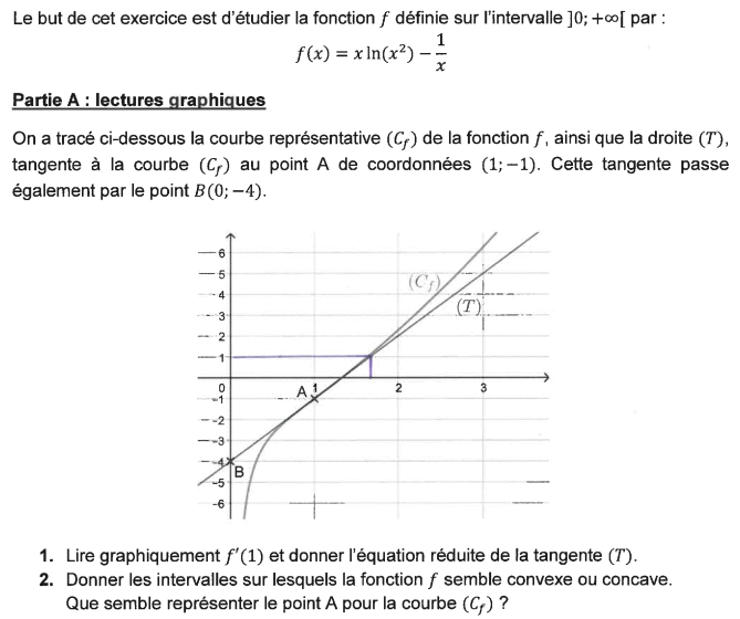
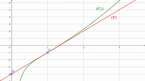
On considère la fonction $\overset{ { \white{ . } } } { f }$ définie sur l'intervalle $\overset{ { \white{ . } } } { ]\,0\;;\;+\infty\,[ }$ par : $\overset{ { \white{ . } } } { f(x)=x\ln(x^2)-\dfrac1x\,. }$

Partie A : lectures graphiques

Bac général spécialité maths 2024 Centres étrangers Jour 1 : image 15

1. Nous devons lire graphiquement $\overset{ { \white{ . } } } { f'(1) }$ et donner l'équation réduite de la tangente $\overset{ { \white{ . } } } { (T). }$

Nous savons que $\overset{ { \white{ . } } } { f'(1) }$ est le coefficient directeur de la tangente $\overset{ { \white{ . } } } { (T)}$
Or nous observons graphiquement que les points $\overset{ { \white{ . } } } { A(1;-1) }$ et $\overset{ { \white{ . } } } { B(0;-4) }$ appartiennent à $\overset{ { \white{ . } } } { (T). }$
Nous en déduisons que :

${ \white{ xxi } }$ $f'(1)=\dfrac{y_B-y_A}{x_B-x_A}=\dfrac{-4-(-1)}{0-1}=\dfrac{-3}{-1}=3.$

D'où $\overset{ { \white{ . } } } { \boxed{f'(1)=3}\,. }$

De plus, l'ordonnée à l'origine de $\overset{ { \white{ . } } } { (T) }$ est égale à -4.
Par conséquent, l'équation réduite de la tangente $\overset{ { \white{ . } } } { (T) }$ est $\overset{ { \white{ . } } } { \boxed{y=3x-4}\,. }$

2. Déterminons les intervalles sur lesquels la fonction $\overset{ { \white{ . } } } { f }$ semble convexe ou concave.

$\overset{ { \white{ . } } }{\bullet}{\white{x}}$ Sur l'intervalle $\overset{ { \white{ . } } } {]0\;;1], }$ la courbe $\overset{ { \white{ . } } } { (C_f) }$ semble être en dessous de la tangente $\overset{ { \white{ . } } } { (T). }$
Nous en déduisons que la fonction $\overset{ { \white{ . } } } { f }$ semble être concave sur l'intervalle $\overset{ { \white{ . } } } {]0;1]. }$

$\overset{ { \white{ . } } }{\bullet}{\white{x}}$ Sur l'intervalle $\overset{ { \white{ . } } } {[1\;;+\infty[, }$ la courbe $\overset{ { \white{ . } } } { (C_f) }$ semble être au-dessus de la tangente $\overset{ { \white{ . } } } { (T). }$
Nous en déduisons que la fonction $\overset{ { \white{ . } } } { f }$ semble être convexe sur l'intervalle $\overset{ { \white{ . } } } {[1\;;+\infty[. }$

Le point $\overset{ { \white{ . } } } { A }$ semble être un point d'inflexion pour la courbe $\overset{ { \white{ . } } } { (C_f). }$

Partie B : étude analytique

Rappelons que pour tout $\overset{ { \white{ . } } } { x>0,\quad f(x)=x\ln(x^2)-\dfrac1x\,. }$

1. Nous devons calculer $\overset{ { \white{ R. } } } { \lim\limits_{x\to+\infty}f(x)}$ et $\overset{ { \white{ R. } } } { \lim\limits_{x\to0}f(x).}$

$\overset{ { \white{ . } } }{\bullet}{\white{x}}$ Calculons $\overset{ { \white{ R. } } } { \lim\limits_{x\to+\infty}f(x).}$

$\left\lbrace\begin{matrix}\left\lbrace\begin{matrix}\lim\limits_{x\to+\infty}x=+\infty\phantom{WW}\\ \overset{ { \phantom{ . } } } { \lim\limits_{x\to+\infty}\ln(x^2)=+\infty}\end{matrix}\right.\\\overset{ { \phantom{ . } } } { \lim\limits_{x\to+\infty}\dfrac1x=0\phantom{WWWW}}\end{matrix}\right.\quad\Longrightarrow\quad\left\lbrace\begin{matrix}\lim\limits_{x\to+\infty}x\ln(x^2)=+\infty\\\overset{ { \phantom{ . } } } { \lim\limits_{x\to+\infty}\dfrac1x=0\phantom{WWWW}}\end{matrix}\right.\\\\\phantom{WWWWWWWWWW}\quad\Longrightarrow\quad\lim\limits_{x\to+\infty}\left(x\ln(x^2)-\dfrac1x\right)=+\infty \\\\\phantom{WWWWWWWWWW}\quad\Longrightarrow\quad\boxed{\lim\limits_{x\to+\infty}f(x)=+\infty}$

$\overset{ { \white{ . } } }{\bullet}{\white{x}}$ Calculons $\overset{ { \white{ R. } } } { \lim\limits_{x\to 0}f(x).}$

$\left\lbrace\begin{matrix}\lim\limits_{x\to0^+}x\ln(x^2)=\lim\limits_{x\to0^+}2x\ln(x)\phantom{WWWWWWWWWWW} \\ \overset{ { \phantom{ . } } } { =0\quad(\text{croissances comparées)}}\\\overset{ { \phantom{ . } } } { \lim\limits_{x\to 0^+}\dfrac1x=+\infty\phantom{WWWWWWWWWWWWWWWWW}}\end{matrix}\right. \quad\Longrightarrow\quad\lim\limits_{x\to0^+}\left(x\ln(x^2)-\dfrac1x\right)=-\infty$

D'où,    $\overset{ { \white{ . } } } {\boxed{\lim\limits_{x\to0}f(x)=-\infty} }$

2. On admet que la fonction $\overset{ { \white{ . } } } { f }$ est deux fois dérivable sur l'intervalle $\overset{ { \white{ . } } } {]\,0\;;\;+\infty\,[. }$

2. a) Déterminons $\overset{ { \white{ . } } } { f'(x) }$ pour $\overset{ { \white{ . } } } { x }$ appartenant à $\overset{ { \white{ . } } } {]\,0\;;\;+\infty\,[. }$

Pour $\overset{ { \white{ . } } } { x }$ appartenant à $\overset{ { \white{ . } } } {]\,0\;;\;+\infty\,[,\quad\boxed{\ln(x^2)=2\ln(x)}\,. }$
Nous déduisons alors que pour tout $\overset{ { \white{ . } } } { x }$ appartenant à $\overset{ { \white{ . } } } {]\,0\;;\;+\infty\,[, }$

${ \white{ xxi } }$ $f'(x)=\Big(x\ln(x^2)\Big)'-\Big(\dfrac1x\Big)'=\Big(2x\ln(x)\Big)'-\Big(\dfrac1x\Big)' \\\overset{ { \phantom{ . } } } { \phantom{f'(x)}=(2x)'\times\ln(x)+2x\times\Big(\ln(x)\Big)'+\dfrac{1}{x^2}} \\\overset{ { \phantom{ . } } } { \phantom{f'(x)}=2\times\ln(x)+2x\times\dfrac{1}{x}+\dfrac{1}{x^2}} \\\overset{ { \phantom{ . } } } { \phantom{f'(x)}=2\ln(x)+2+\dfrac{1}{x^2}} \\\\\Longrightarrow\quad\boxed{\forall\,x\in\,]\,0\;;\;+\infty\,[,\;f'(x)=2\ln(x)+2+\dfrac{1}{x^2}}$

2. b) Déterminons $\overset{ { \white{ . } } } { f''(x) }$ pour tout $\overset{ { \white{ . } } } { x }$ appartenant à $\overset{ { \white{ . } } } {]\,0\;;\;+\infty\,[. }$

Pour tout $\overset{ { \white{ . } } } { x }$ appartenant à $\overset{ { \white{ . } } } {]\,0\;;\;+\infty\,[,}$

${ \white{ xxi } }$ $f''(x)=\left(2\ln(x)+2+\dfrac{1}{x^2}\right)' \\ \overset{ { \phantom{ . } } } { \phantom{f''(x)}=\dfrac2x+0-\dfrac{2}{x^3}} \\ \overset{ { \phantom{ . } } } { \phantom{f''(x)}=\dfrac2x-\dfrac{2}{x^3}} \\ \overset{ { \phantom{ . } } } { \phantom{f''(x)}=\dfrac{2x^2-2}{x^3}} \\ \overset{ { \phantom{ . } } } { \phantom{f''(x)}=\dfrac{2(x^2-1)}{x^3}} \\ \overset{ { \phantom{ . } } } { \phantom{f''(x)}=\dfrac{2(x+1)(x-1)}{x^3}} \\\\\Longrightarrow\quad\boxed{\forall\,x\in\,]\,0\;;\;+\infty\,[,\;f''(x)=\dfrac{2(x+1)(x-1)}{x^3}}$

3. a) Nous devons étudier la convexité de la fonction $\overset{ { \white{ . } } } { f }$ sur l'intervalle $\overset{ { \white{ . } } } {]\,0\;;\;+\infty\,[. }$

Étudions le signe de $\overset{ { \white{ . } } } {f''(x) }$ sur l'intervalle $\overset{ { \white{ . } } } {]\,0\;;\;+\infty\,[. }$

Pour tout $\overset{ { \white{ . } } } { x }$ appartenant à $\overset{ { \white{ . } } } {]\,0\;;\;+\infty\,[,}$ nous avons : $\overset{ { \white{ . } } } { 2(x+1)>0 }$ et ${ x^3>0. }$

Dès lors, le signe de $\overset{ { \white{ . } } } { f''(x) }$ est le signe de $\overset{ { \white{ . } } } { (x-1) }$

${ \phantom{ xxi } }\begin{matrix}x-1<0\Longleftrightarrow x<1\\\overset{ { \white{.} } } {x-1=0\Longleftrightarrow x=1} \\\overset{ { \phantom{.} } } {x-1>0\Longleftrightarrow x>1}\end{matrix} \begin{matrix} \\||\\||\\||\\||\\||\\||\\||\\||\\||\\|| \\\phantom{WWW}\end{matrix} \begin{array}{|c|ccccccc|}\hline &&&&&&&&x&0&&&1&&&+\infty &&&&&&&& \\\hline &&&&&&&\\x-1&&-&-&0&+&+&\\&&&&&&&\\\hline&|&&&&&&\\f''(x)&|&-&-&0&+&+&\\&|&&&&&&\\\hline \end{array}$

Nous pouvons en déduire la convexité de $\overset{ { \white{ . } } } { f }$ sur l'intervalle $\overset{ { \white{ . } } } {]\,0\;;\;+\infty\,[. }$

$\begin{array}{|c|ccccc|} \hline &&&&&\\x & 0 & & 1 & &+\infty \\ & & & & & \\ \hline &| && & & \\ f''(x) &| &-&0& + & \\ &| & & & & \\ \hline &| &&| & & \\ \text{Convexité de f} & |&\text{concave}&|& \text{convexe} & \\ &| & &| & & \\ \hline \end{array}$

La fonction $\overset{ { \white{ . } } } { f }$ est concave sur $\overset{ { \white{ . } } } { ]0\;;\;1[ }$ et est convexe sur $\overset{ { \white{ . } } } { ]1\;;\;+\infty[. }$

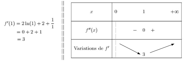
3. b) Nous devons étudier les variations de la fonction $\overset{ { \white{ . } } } { f' }$ , puis le signe de $\overset{ { \white{ . } } } { f'(x) }$ sur l'intervalle $\overset{ { \white{ . } } } {]\,0\;;\;+\infty\,[. }$

En nous aidant de la question 3. a), nous obtenons les variations de la fonction $\overset{ { \white{ . } } } { f'. }$

${ \phantom{ xxi } }\begin{matrix}f'(1)=2\ln(1)+2+\dfrac11\\\overset{ { \white{.} } } {=0+2+1} \\\overset{ { \phantom{.} } } {=3\phantom{WWW}}\end{matrix} \begin{matrix} \\||\\||\\||\\||\\||\\||\\||\\||\\||\\||\\\phantom{WWW}\end{matrix} \begin{array}{|c|ccccccc|} \hline &&&&&&&&x&0&&&1&&&+\infty &&&&&&&& \\\hline &|&&&&&&\\f''(x)&|&-&-&0&+&+&\\&|&&&&&&\\\hline&|&&&&&&\\\text{Variations de }f'&|&\searrow&\searrow&&\nearrow&\nearrow&\\&|&&&3&&&\\\hline \end{array}$

Nous remarquons que 3 est le minimum de $\overset{ { \white{ . } } } { f' }$ sur l'intervalle $\overset{ { \white{ . } } } {]\,0\;;\;+\infty\,[. }$

Par conséquent, pour tout $\overset{ { \white{ . } } } { x }$ appartenant à $\overset{ { \white{ . } } } {]\,0\;;\;+\infty\,[,}$    $\overset{ { \white{ . } } } { f'(x)>0 }$ et par suite, la fonction $\overset{ { \white{ . } } } { f }$ est strictement croissante sur $\overset{ { \white{ . } } } {]\,0\;;\;+\infty\,[.}$

4. a) Montrons que l'équation $\overset{ { \white{ . } } } { f(x)=0 }$ admet une unique solution $\overset{ { \white{ . } } } { \alpha }$ sur l'intervalle $\overset{ { \white{ . } } } {]\,0\;;\;+\infty\,[.}$

La fonction $\overset{ { \white{ . } } } {f }$ est continue est strictement croissante sur l'intervalle $\overset{ { \white{ . } } } {]\,0\;;\;+\infty\,[.}$

De plus, $\overset{ { \white{ . } } } { \left\lbrace\begin{matrix}\lim\limits_{x\to 0^+}f=-\infty\\ \overset{ { \phantom{ . } } } {\lim\limits_{x\to+\infty}f=+\infty}\end{matrix}\right.\quad\Longrightarrow\quad \boxed{0\in\;]\lim\limits_{x\to 0^+}f\;;\;\lim\limits_{x\to+\infty}f\,[} }$

Par le corollaire du théorème des valeurs intermédiaires, il existe un unique réel $\overset{ { \white{ . } } } { \alpha\in\,]\,0\;;\;+\infty\,[ }$ tel que $\overset{ { \white{ . } } } { f(\alpha)=0. }$
Par conséquent, l'équation $\overset{ { \white{ . } } } { f(x)=0 }$ admet une unique solution $\overset{ { \white{ . } } } { \alpha }$ sur l'intervalle $\overset{ { \white{ . } } } {]\,0\;;\;+\infty\,[.}$

4. b) Par la calculatrice, nous obtenons $\overset{ { \white{ . } } } { \alpha\approx 1,33 }$ (valeur arrondie à 10^-2 près).

${ \white{ xxi } }$ $f(\alpha)=0\quad\Longleftrightarrow\quad \alpha\ln(\alpha^2)-\dfrac{1}{\alpha}=0 \\ \overset{ { \phantom{ . } } } { \phantom{f(\alpha)=0}\quad\Longleftrightarrow\quad \alpha\ln(\alpha^2)=\dfrac{1}{\alpha}} \\ \overset{ { \phantom{ . } } } { \phantom{f(\alpha)=0}\quad\Longleftrightarrow\quad \ln(\alpha^2)=\dfrac{1}{\alpha^2}} \\ \overset{ { \phantom{ . } } } { \phantom{f(\alpha)=0}\quad\Longleftrightarrow\quad \boxed{\alpha^2=\exp\left(\dfrac{1}{\alpha^2}\right)}}$

6 points

exercice 4

Pour tout entier naturel $\overset{ { \white{ . } } } { n, }$ on considère les intégrales suivantes :

$\overset{ { \white{ . } } } { I_n=\displaystyle\int_0^{\pi}\text e^{-nx}\sin(x)\,\text dx}$ et $\overset{ { \white{ . } } } { J_n=\displaystyle\int_0^{\pi}\text e^{-nx}\cos(x)\,\text dx.}$

1. Nous devons calculer $\overset{ { \white{ . } } } { I_0. }$

${ \white{ xxi } }$ ${ \white{ xxi } }$ $\overset{ { \white{ . } } } { I_0=\displaystyle\int_0^{\pi}\text e^{0}\sin(x)\,\text dx} \\\overset{ { \phantom{ . } } } { \phantom{I_0}=\displaystyle\int_0^{\pi}\sin(x)\,\text dx} \\\overset{ { \phantom{ . } } } { \phantom{I_0}=\left[\overset{}{-\cos(x)}\right]}_0^{\pi} \\\overset{ { \phantom{ . } } } { \phantom{I_0}=-\cos(\pi)-(-\cos(0))} \\\overset{ { \phantom{ . } } } { \phantom{I_0}=-(-1)-(-1)} \\\overset{ { \phantom{ . } } } { \phantom{I_0}=2} \\\\\Longrightarrow\quad\boxed{I_0=2}$

2. a) Montrons que pour tout entier naturel $\overset{ { \white{ o. } } }{ n, }$ nous avons $\overset{ { \white{ . } } } { I_n\ge0. }$

$\overset{ { \white{ . } } }{\bullet}{\white{x}}$ Nous savons que la fonction exponentielle est strictement positive.
${ \white{ xi } }$ Dès lors, sur l'intervalle $\overset{ { \white{ . } } } { [0\;;\;\pi],\quad\text e^{-nx}>0. }$

$\overset{ { \white{ . } } }{\bullet}{\white{x}}$ Sur l'intervalle $\overset{ { \white{ . } } } { [0\;;\;\pi],\quad\sin(x)\ge0. }$

D'où, sur l'intervalle $\overset{ { \white{ . } } } { [0\;;\;\pi],\quad\text e^{-nx}\sin(x)\ge0. }$
Par la positivité de l'intégrale, nous en déduisons que $\overset{ { \white{ . } } } { \displaystyle\int_0^{\pi}\text e^{-n^x}\sin(x)\,\text dx\ge0 }$
Par conséquent, $\overset{ { \white{ . } } } {\boxed{\forall\,n\in\N,\quad I_n\ge0}\,. }$

2. b) Montrons que pour tout entier naturel $\overset{ { \white{ o. } } } { n, }$ nous avons $\overset{ { \white{ . } } } { I_{n+1}-I_n\le0. }$

${ \white{ xxi } }$ $\overset{ { \white{ . } } } { I_{n+1}-I_n=\displaystyle\int_0^{\pi}\text e^{-(n+1)x}\sin(x)\,\text dx-\displaystyle\int_0^{\pi}\text e^{-nx}\sin(x)\,\text dx} \\\overset{ { \white{ . } } } { \phantom{I_{n+1}-I_n}=\displaystyle\int_0^{\pi}\Big(\text e^{-(n+1)x}\sin(x)-\text e^{-nx}\sin(x)\Big)\,\text dx} \\\overset{ { \phantom{ . } } } { \phantom{I_{n+1}-I_n}=\displaystyle\int_0^{\pi}\Big(\text e^{-nx}\text e^{-x}\sin(x)-\text e^{-nx}\sin(x)\Big)\,\text dx} \\\\\Longrightarrow { I_{n+1}-I_n=\displaystyle\int_0^{\pi}\text e^{-nx}\sin(x)\Big(\text e^{-x}-1\Big)\,\text dx}$

Or pour tout $\overset{ { \white{ . } } } { x\in[0\;;\;\pi], }$

${ \white{ xxi } }$ $\overset{ { \white{ . } } }{\bullet}{\white{x}}$ $\overset{ { \white{ . } } } { \text e^{-nx}>0 }$

${ \white{ xxi } }$ $\overset{ { \white{ . } } }{\bullet}{\white{x}}$ $\overset{ { \white{ . } } } { \sin(x)\ge 0 }$

${ \white{ xxi } }$ $\overset{ { \white{ . } } }{\bullet}{\white{x}}x\ge0\quad\Longrightarrow\quad -x\le 0 \\ \overset{ { \phantom{ . } } } {\phantom{WWwx} \quad\Longrightarrow\quad \text e^{-x}\le \text e^0} \\ \overset{ { \phantom{ . } } } {\phantom{WWwx} \quad\Longrightarrow\quad \text e^{-x}\le 1} \\ \overset{ { \phantom{ . } } } {\phantom{WWwx} \quad\Longrightarrow\quad \text e^{-x}-1\le 0}$

Nous en déduisons que $\overset{ { \white{ . } } } {\text e^{-nx}\sin(x)\Big(\text e^{-x}-1\Big) \le 0 .}$
L'intégrale d'une fonction négative sur un intervalle est négative.
Par conséquent, $\overset{ { \white{ . } } } { \boxed{\forall\,n\in\N,\quad I_{n+1}-I_n\le0}\,. }$

2. c) Nous avons montré dans la question 2. b) que la suite $\overset{ { \white{ . } } } { (I_n) }$ est décroissante.
Nous avons également montré dans la question 2. a) que la suite $\overset{ { \white{ . } } } { (I_n) }$ est minorée par 0.

D'après le théorème de convergence monotone, nous en déduisons que la suite $\overset{ { \white{ . } } } { (I_n) }$ est convergente.

3. a) Montrons que pour tout entier naturel $\overset{ { \white{ o. } } } { n, }$ nous avons : $\overset{ { \white{ . } } } { I_n\le \displaystyle\int_0^{\pi}\text e^{-nx}\,\text dx. }$

Pour tout $\overset{ { \white{ . } } } { x\in[0\;;\;\pi], }$

${ \white{ xxi } }$ $\sin(x)\le1\quad\Longrightarrow\quad\text e^{-nx}\sin(x)\le\text e^{-nx}\enskip\enskip\quad\text{car } \text e^{-nx}>0 \\ \overset{ { \phantom{ . } } } { \phantom{\sin(x)\le1}\quad\Longrightarrow\quad\displaystyle\int_0^{\pi}\text e^{-nx}\sin(x)\,\text dx\le\displaystyle\int_0^{\pi}\text e^{-nx}\,\text dx.} \\\\\Longrightarrow\quad\boxed{\forall\,n\in\N,\quad I_n\le\displaystyle\int_0^{\pi}\text e^{-nx}\,\text dx}$

3. b) Montrons que pour tout entier naturel $\overset{ { \white{ . } } } { n\ge1, }$ nous avons : $\overset{ { \white{ . } } } { \displaystyle\int_0^{\pi}\text e^{-nx}\,\text dx=\dfrac{1-\text e^{-n\pi}}{n}. }$

Pour tout entier naturel $\overset{ { \white{ . } } } { n\ge1, }$ nous avons :

${ \white{ xxi } }$ $\displaystyle\int_0^{\pi}\text e^{-nx}\,\text dx=\left[\dfrac{\text e^{-nx}}{-n}\right]_0^{\pi} \\ \overset{ { \phantom{ . } } } { \phantom{\displaystyle\int_0^{\pi}\text e^{-nx}\,\text dx}=\dfrac{\text e^{-n\pi}}{-n}-\dfrac{\text e^{0}}{-n}} \\ \overset{ { \phantom{ . } } } { \phantom{\displaystyle\int_0^{\pi}\text e^{-nx}\,\text dx}=\dfrac{-\text e^{-n\pi}}{n}+\dfrac{1}{n}} \\ \overset{ { \phantom{ . } } } { \phantom{\displaystyle\int_0^{\pi}\text e^{-nx}\,\text dx}=\dfrac{1-\text e^{-n\pi}}{n}} \\\\\Longrightarrow\quad\boxed{\forall\,n\in\N,\;n\ge1,\quad \overset{ { \white{ . } } } { \displaystyle\int_0^{\pi}\text e^{-nx}\,\text dx=\dfrac{1-\text e^{-n\pi}}{n}} }$

3. c) Nous devons calculer la limite de la suite $\overset{ { \white{ . } } } { (I_n). }$

En utilisant les questions précédentes, nous obtenons pour tout entier naturel $\overset{ { \white{ . } } } { n\ge1 }$ :

${ \white{ xxi } }$ $\left\lbrace\begin{matrix}I_n\ge 0\phantom{WWWWWW}\\ \overset{ { \phantom{ . } } } { I_n\le{\red{\displaystyle\int_0^{\pi}\text e^{-nx}\,\text dx}}}\phantom{WWW}\\ {\red{ \overset{ { \phantom{ . } } } { \displaystyle\int_0^{\pi}\text e^{-nx}\,\text dx}}} =\dfrac{1-\text e^{-n\pi}}{n}\end{matrix}\right.\quad\Longrightarrow\quad\boxed{0\le I_n\le\dfrac{1-\text e^{-n\pi}}{n}}$

Calculons ${ \lim\limits_{n\to+\infty}\dfrac{1-\text e^{-n\pi}}{n} }$

$\left\lbrace\begin{matrix}\lim\limits_{n\to+\infty}(-n\pi)=-\infty\\\lim\limits_{X\to-\infty}\text e^X=0\phantom{WW}\end{matrix}\right.\quad\Longrightarrow\quad\lim\limits_{n\to+\infty}\text e^{-n\pi}=0 \\ \overset{ { \phantom{ . } } } { \phantom{WWWWWWWWW}\quad\Longrightarrow\quad\lim\limits_{n\to+\infty}(1-\text e^{-n\pi})=1} \\ \overset{ { \phantom{ . } } } { \phantom{WWWWWWWWW}\quad\Longrightarrow\quad\boxed{\lim\limits_{n\to+\infty}\dfrac{1-\text e^{-n\pi}}{n} =0}}$

En utilisant le théorème d'encadrement (théorème des gendarmes), nous obtenons :

${ \white{ xxi } }$ $\left\lbrace\begin{matrix}0\le I_n\le\dfrac{1-\text e^{-n\pi}}{n}\\\overset{ { \white{ . } } } { \lim\limits_{n\to+\infty}\dfrac{1-\text e^{-n\pi}}{n}=0}\end{matrix}\right.\quad\Longrightarrow\quad\boxed{\lim\limits_{n\to+\infty}I_n=0}$

4. a) Nous devons montrer que pour tout entier naturel $\overset{ { \white{ . } } } { n\ge1, }$

$\overset{ { \white{ . } } } { I_n=1+\text e^{-n\pi}-n\,J_n }$ ${ \white{ xxi } }$ et ${ \white{ xxi } }$ $\overset{ { \white{ . } } } { I_n=\dfrac1n\,J_n. }$

$\overset{ { \white{ . } } }{\bullet}{\white{x}}$ Montrons que $\overset{ { \white{ . } } } {I_n=1+\text e^{-n\pi}-n\,J_n .}$

Calculons $\overset{ { \white{ . } } } { I_n=\displaystyle\int_{0}^{\pi} \text e^{-nx}\,\sin(x)\,\text{d}x. }$

$\underline{\text{Formule de l'intégrale par parties}}\ :\ {\blue{\displaystyle\int_0^{\pi}u(x)v'(x)\,\text{d}x=\left[\overset{}{u(x)v(x)}\right]\limits_0^{\pi}- \displaystyle\int\limits_0^{\pi}u'(x)v(x)\,\text{d}x}}. \\ \\ \left\lbrace\begin{matrix}u(x)=\text e^{-nx}\quad\Longrightarrow\quad u'(x)=-n\text e^{-nx} \\\\v'(x)=\sin(x)\phantom{}\quad\Longrightarrow\quad v(x)=-\cos(x)\end{matrix}\right.$

$\text{Dès lors }\;\overset{ { \white{ . } } } { \displaystyle\int_{0}^{\pi} \text e^{-nx}\,\sin(x)\,\text{d}x=\left[\overset{}{\text e^{-nx}\Big(-\cos(x)\Big)\,}\right]_0^{\pi}-\displaystyle\int_0^{\pi}(-n\text e^{-nx})\times\Big(-\cos(x)\Big)\,\text{d}x} \\\overset{ { \white{ . } } } {\phantom{WWWWWWWWWW}=\left[\overset{}{-\text e^{-nx}\,\cos(x)}\right]_0^{\pi}-n\displaystyle\int_0^{\pi}\text e^{-nx}\,\cos(x)\,\text{d}x} \\\overset{ { \phantom{ . } } } {\phantom{WWWWWWWWWW}=\Big(-\text e^{-n\pi}\cos(\pi)+\text e^{0}\cos(0)\Big)-n\,J_n} \\\overset{ { \white{ . } } } {\phantom{WWWWWWWWWW}=\text e^{-n\pi}+1-n\,J_n}$

Par conséquent, $\boxed{I_n=1+\text e^{-n\pi}-n\,J_n}$

$\overset{ { \white{ . } } }{\bullet}{\white{x}}$ Montrons que $I_n=\dfrac1n\,J_n .$

Calculons $\overset{ { \white{ . } } } { I_n=\displaystyle\int_{0}^{\pi} \sin(x)\,\text e^{-nx}\,\text{d}x. }$

$\underline{\text{Formule de l'intégrale par parties}}\ :\ {\blue{\displaystyle\int_0^{\pi}u(x)v'(x)\,\text{d}x=\left[\overset{}{u(x)v(x)}\right]\limits_0^{\pi}- \displaystyle\int\limits_0^{\pi}u'(x)v(x)\,\text{d}x}}. \\ \\ \left\lbrace\begin{matrix}u(x)=\sin(x)\quad\Longrightarrow\quad u'(x)=\cos(x) \\\\v'(x)=\text e^{-nx}\phantom{}\quad\Longrightarrow\quad v(x)=\dfrac{\text e^{-nx}}{-n}\end{matrix}\right.$

$\text{Dès lors }\;\overset{ { \phantom{ . } } } { \displaystyle\int_{0}^{\pi} \sin(x)\text e^{-nx}\,\text{d}x=\left[\overset{}{\sin(x)\,\dfrac{\text e^{-nx}}{-n}}\right]_0^{\pi}-\displaystyle\int_0^{\pi}\cos(x)\,\dfrac{\text e^{-nx}}{-n}\,\text{d}x} \\\overset{ { \phantom{ . } } } {\phantom{WWWWWWWWWW}=\left[\overset{}{\sin(x)\,\dfrac{\text e^{-nx}}{-n}}\right]_0^{\pi}+\dfrac1n\displaystyle\int_0^{\pi}\cos(x)\,\text e^{-nx}\,\text{d}x} \\\overset{ { \phantom{ . } } } {\phantom{WWWWWWWWWW}=\Big(\sin(\pi)\,\dfrac{\text e^{-n\pi}}{-n}-\sin(0)\,\dfrac{\text e^{0}}{-n}\Big)+\dfrac1n\,J_n} \\\overset{ { \phantom{ . } } } {\phantom{WWWWWWWWWW}=\Big(0-0\Big)+\dfrac1n\,J_n} \\\overset{ { \phantom{ . } } } {\phantom{WWWWWWWWWW}=\dfrac1n\,J_n}$

Par conséquent, $\boxed{I_n=\dfrac1n\,J_n}$

4. b) Pour tout entier naturel $\overset{ { \white{ . } } } { n\ge1, }$

${ \white{ xxi } }$ $\left\lbrace\begin{matrix} I_n=1+\text e^{-n\pi}-n\,J_n \\ I_n=\dfrac1n\,J_n\phantom{WWWyW}\end{matrix}\right.\quad\Longrightarrow\quad \left\lbrace\begin{matrix} n\,J_n=1+\text e^{-n\pi} -I_n\\n\,J_n=n^2\,I_n\phantom{WWyW}\end{matrix}\right. \\ \overset{ { \phantom{ . } } } {\phantom{WWWWWWWxWW}\quad\Longrightarrow\quad 1+\text e^{-n\pi} -I_n=n^2\,I_n } \\ \overset{ { \phantom{ . } } } {\phantom{WWWWWWWxWW}\quad\Longrightarrow\quad 1+\text e^{-n\pi}=I_n+n^2\,I_n } \\ \overset{ { \phantom{ . } } } {\phantom{WWWWWWWxWW}\quad\Longrightarrow\quad 1+\text e^{-n\pi}=(1+n^2)\,I_n } \\\\\Longrightarrow\quad\boxed{\forall\,n\in\N,\;n\ge1,\quad I_n=\dfrac{1+\text e^{-n\pi}}{n^2+1}}$

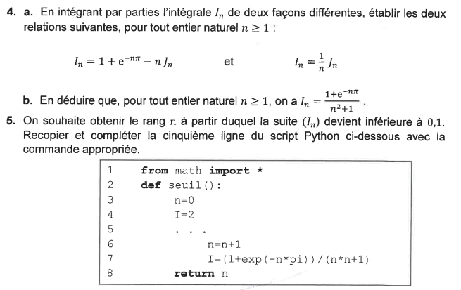
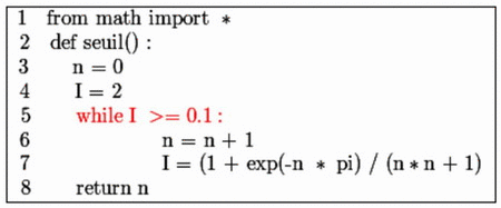
5. On souhaite obtenir le rang n à partir duquel la suite $\overset{ { \white{ . } } } { (I_n) }$ devient inférieure à 0,1.
Ci-dessous le script Python permettant d'obtenir le rang n.

Bac général spécialité maths 2024 Centres étrangers Jour 1 : image 16

Publié par malou le 11-06-2024

ceci n'est qu'un extrait
Pour visualiser la totalité des cours vous devez vous inscrire / connecter (GRATUIT)
Inscription Gratuite se connecter

Merci à / pour avoir contribué à l'élaboration de cette fiche

Cette fiche

Voir la correction
Imprimer
Réduire / Agrandir
Pour plus d'options, Connectez vous
Forum de maths

forum de terminale
Plus de 147 208 topics de mathématiques en terminale sur le forum.