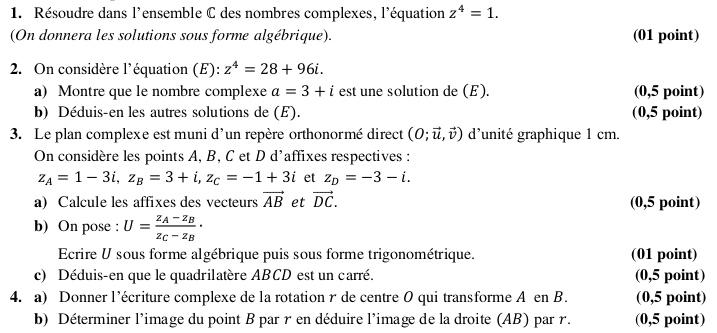
1. Résoudre dans l'ensemble des nombres complexes, l'équation .
D'où l'ensemble des solutions de l'équation est
2. On considère l'équation .
2. a) Nous devons montrer que le nombre complexe est une solution de .
Montrons que .
Par conséquent, le nombre complexe est une solution de .
2. b) Nous devons en déduire les autres solutions de .
Nous avons montré que est une solution de en montrant que .
Donc pour toute autre solution de , nous obtenons : .
Soit .
Nous obtenons alors : , et par suite, doit être une solution de l'équation .
Ces solutions ont été identifiées dans la question 1.
Nous obtenons ainsi:
soit
soit
soit
soit
D'où les autres solutions de sont et .
Par conséquent, l'ensemble des solutions de l'équation est
3. Le plan complexe est muni d'un repère orthonormé direct d'unité graphique 1 cm.
On considère les points et d'affixes respectives : et
3. a) Nous devons calculer les affixes des vecteurs et .
3. b) On pose : . Nous devons écrire sous forme algébrique puis sous forme trigonométrique.
Écrivons sous forme algébrique.
Écrivons sous forme trigonométrique.
3. c) Nous devons en déduire que le quadrilatère est un carré.
Montrons que le quadrilatère est un parallélogramme.
Donc le quadrilatère est un parallélogramme.
Montrons que le triangle est rectangle et isocèle en .
D'une part, nous obtenons :
D'autre part,
Donc les droites et sont perpendiculaires.
Nous en déduisons que le triangle est rectangle et isocèle en .
Par conséquent, le quadrilatère est un carré.
4. a) Nous devons donner l'écriture complexe de la rotation de centre qui transforme en .
L'écriture complexe de la rotation est de la forme : .
D'où l'écriture complexe de la rotation de centre qui transforme en est
4. b) Nous devons déterminer l'image du point par et en déduire l'image de la droite par .
D'où l'image de par la rotation est le point .
D'où l'image de par la rotation est le point .
Nous en déduisons que l'image de la droite par la rotation est la droite .
5 points
exercice 2
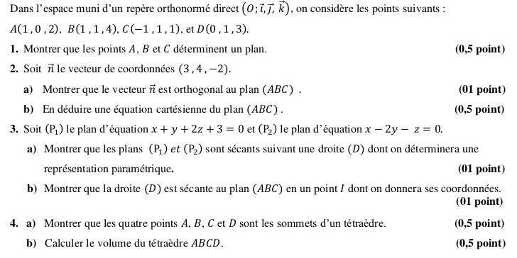
Dans l'espace muni d'un repère orthonormé direct , on considère les points et .
1. Nous devons montrer que les points et déterminent un plan.
Montrons que les vecteurs et ne sont pas colinéaires.
Manifestement, les vecteurs et ne sont pas colinéaires.
Dès lors, les points et ne sont pas alignés.
Par conséquent, les points et déterminent un plan.
2. Soit le vecteur de coordonnées .
2. a) Nous devons montrer que le vecteur est orthogonal au plan .
Dès lors, le vecteur est orthogonal à deux vecteurs et non colinéaires du plan .
Il s'ensuit que le vecteur est normal au plan .
2. b) Nous devons en déduire une équation cartésienne du plan .
Nous avons montré dans la question précédente que le vecteur est normal au plan .
D'où l'équation du plan est de la forme où est un nombre réel.
Nous savons que appartient à ce plan .
Donc soit
Par conséquent, une équation cartésienne du plan est
3. Soit le plan d'équation et le plan d'équation .
3. a) Nous devons montrer que les plans et sont sécants suivant une droite dont on déterminera une représentation paramétrique.
Les plans et sont sécants si leurs vecteurs normaux ne sont pas colinéaires.
Un vecteur normal de est et un vecteur normal de est
Les coordonnées des deux vecteurs ne sont pas proportionnelles.
Les vecteurs ne sont donc pas colinéaires.
Par conséquent, les plans et sont sécants suivant une droite .
Déterminons une représentation paramétrique de la droite .
Le point de vérifie le système suivant :
Choisissons comme paramètre et posons .
Nous obtenons ainsi :
Par conséquent, une représentation paramétrique de la droite est
3. b) Nous devons montrer que la droite est sécante au plan en un point dont on donnera ses coordonnées.
Montrons qu'il existe un nombre réel tel que .
En effet,
En remplaçant par dans la représentation paramétrique de , nous obtenons :
D'où, les coordonnées du point sont
4. a) Nous devons montrer que les quatre points et sont les sommets d'un tétraèdre.
Montrons que le point n'appartient pas au plan en montrant que ses coordonnées ne vérifient pas l'équation cartésienne de .
En effet,
Donc les quatre points et ne sont pas coplanaires.
Nous en déduisons que les quatre points et sont les sommets d'un tétraèdre.
4. b) Nous devons calculer le volume en unité de volume (u.v.) du tétraèdre .
Nous savons que
Nous obtenons ainsi :
Nous en déduisons que :
10 points
probleme
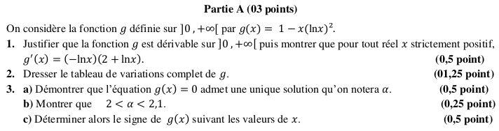
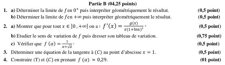
On considère la fonction définie sur par .
On note la courbe représentative de dans le plan muni d'un repère orthonormé d'unité graphique 2 cm.
Partie A
On considère la fonction définie sur par .
1. Nous devons justifier que la fonction est dérivable sur puis montrer que pour tout réel strictement positif, .
La fonction est la somme de produits de fonctions dérivables sur .
Donc la fonction est dérivable sur .
Pour tout ,
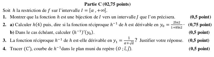
2. Nous devons dresser le tableau de variations complet de .
Par définition, la fonction est définie sur . Calculons .
Calculons .
Nous pouvons ainsi dresser le tableau de signes de sur .
D'où le tableau de variations de .
3. a) Nous devons démontrer que l'équation admet une unique solution qu'on notera .
Sur l'intervalle :
Le tableau de variations de montre que sur l'intervalle , cette fonction admet un minimum égal à .
Dès lors, sur l'intervalle , l'équation n'admet pas de solution.
Sur l'intervalle :
La fonction est continue et strictement décroissante sur l'intervalle .
De plus,
Par le corollaire du théorème des valeurs intermédiaires, il existe un unique réel tel que .
En conclusion, l'équation admet une solution unique dans l'intervalle .
3. b) Montrons que .
3. c) Nous devons déterminer le signe de suivant les valeurs de .
En nous aidant du tableau de variations de , nous en déduisons que :
.
Partie B
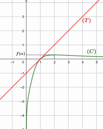
1. a) Nous devons déterminer la limite de en , puis interpréter géométriquement le résultat.
Géométriquement, ce résultat signifie que la courbe admet une asymptote verticale d'équation .
1. b) Nous devons déterminer la limite de en , puis interpréter géométriquement le résultat.
Pour tout
Nous obtenons ainsi :
Géométriquement, ce résultat signifie que la courbe admet une asymptote horizontale en d'équation .
2. a) Montrons que pour tout , on a : .
Pour tout ,
2. b) Nous devons étudier le sens de variation de , puis dresser son tableau de variation.
Nous observons que le signe de sur l'intervalle est le signe de car pour tout .
Or le signe de a été étudié dans la question 3. c) - Partie A.
Dès lors,
.
Nous en déduisons que la fonction est croissante sur l'intervalle et est décroissante sur l'intervalle .
Nous pouvons ainsi dresser le tableau de variation de .
2. c) Nous devons vérifier que .
Nous savons que est l'unique solution de l'équation .
Donc nous obtenons :
Il s'ensuit que :
3. Déterminons une équation de la tangente à au point d'abscisse .
Une équation de la tangente est de la forme .
Or
Par conséquent, une équation de la tangente à au point d'abscisse est
4. Nous devons construire et .
Partie C
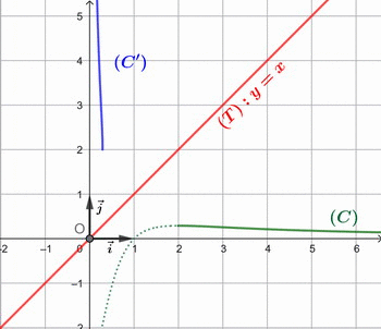
Soit la restriction de sur l'intervalle .
1. Nous devons montrer que la fonction est une bijection de vers un intervalle que l'on précisera.
La fonction est continue et strictement décroissante sur l'intervalle avec et La fonction réalise donc une bijection de sur
2. a) Nous devons calculer puis, dire si la fonction de est dérivable en .
Montrons que la fonction est dérivable en en montrant que .
En effet, .
Par conséquent, la fonction est dérivable en .
2. b) Calculons .
3. Déterminons si la fonction réciproque de est dérivable en .
Nous savons que .
Or nous avons montré dans la question 2. b) - Partie B que , soit que .
Nous en déduisons que la fonction réciproque de n'est pas dérivable en .
4. Traçons , courbe de dans le plan muni du repère .
Le graphique de la fonction réciproque de est le symétrique de la courbe par rapport à l'axe d'équation .
Merci à Hiphigenie et malou pour l'élaboration de cette contribution.
Publié par malou
le
ceci n'est qu'un extrait
Pour visualiser la totalité des cours vous devez vous inscrire / connecter (GRATUIT) Inscription Gratuitese connecter
Merci à Hiphigenie / malou pour avoir contribué à l'élaboration de cette fiche
Désolé, votre version d'Internet Explorer est plus que périmée ! Merci de le mettre à jour ou de télécharger Firefox ou Google Chrome pour utiliser le site. Votre ordinateur vous remerciera !

 des nombres complexes, l'équation
  .
.


: z^4 = 28 + 96\text i }) .
. est une solution de
  }) .
. .
.^4 \\\overset{ { \white{ . } } } { \phantom{ a=3+\text i}\quad\Longrightarrow\quad a^4=\Big((3+\text i)^2\Big)^2} \\\overset{ { \white{ . } } } { \phantom{ a=3+\text i}\quad\Longrightarrow\quad a^4=(9+6\text i-1)^2} \\\overset{ { \white{ . } } } { \phantom{ a=3+\text i}\quad\Longrightarrow\quad a^4=(8+6\text i)^2} )

 : z^4=28+96\text i }) en montrant que
en montrant que  .
. de
de  }) , nous obtenons :
, nous obtenons :  .
. \\\overset{ { \white{ . } } } { \phantom{ \text{Or }\quad z^4=a^4}\quad\Longleftrightarrow\quad \left(\dfrac{z}{a}\right)^4=1 } )
 .
.^4=1 \quad\Longleftrightarrow\quad Z^4=1 }) , et par suite,
, et par suite,  doit être une solution de l'équation
  .
.


\quad\text{ou}\quad z=-\text i(3+\text i) )

 et
et  .
.: z^4=28+96\text i }) est
est }=\lbrace3+\text i\;;\;-3-\text i\;;\;-1+3\text i\;;\;1-3\text i\rbrace} })
 }) d'unité graphique 1 cm.
d'unité graphique 1 cm. et
et  d'affixes respectives :
 et
et 
 et
et  .
. 
-(1-3\text i) } \\\overset{ { \white{ . } } } { \phantom{z_{\overrightarrow{AB}}}=3+\text i-1+3\text i } \\\overset{ { \white{ . } } } { \phantom{z_{\overrightarrow{AB}}}=2+4\text i } \\\\\quad\Longrightarrow\quad\boxed{z_{\overrightarrow{AB}}=2+4\text i } )
-(-3-\text i) } \\\overset{ { \white{ . } } } { \phantom{z_{\overrightarrow{AB}}}=-1+3\text i+3+\text i } \\\overset{ { \white{ . } } } { \phantom{z_{\overrightarrow{AB}}}=2+4\text i } \\\\\quad\Longrightarrow\quad\boxed{z_{\overrightarrow{DC}}=2+4\text i } )
 .
. sous forme algébrique puis sous forme trigonométrique.
  Écrivons
  sous forme algébrique.
-(3+\text i)}{(-1+3\text i)-(3+\text i)} } \\\overset{ { \white{ . } } } { \phantom{ U}=\dfrac{1-3\text i-3-\text i}{-1+3\text i-3-\text i} } \\\overset{ { \white{ . } } } { \phantom{ U}=\dfrac{-2-4\text i}{-4+2\text i} } )
}{-4+2\text i} } \\\overset{ { \white{ . } } } { \phantom{ U}=\dfrac{\text i(-4+2\text i)}{-4+2\text i} } \\\overset{ { \white{ . } } } { \phantom{ U}=\text i} \\\\\Longrightarrow\quad\boxed{U=\text i} )
+\text i\sin\left(\dfrac{\pi}{2}\right)} )
 est un carré.
 est rectangle et isocèle en
  .
.
![U=\dfrac{z_A-z_B}{z_C-z_B}=\text i\quad\Longleftrightarrow\quad \arg\left(\dfrac{z_A-z_B}{z_C-z_B}\right)\equiv \arg(\text i) \;[2\pi]\\\overset{ { \white{ . } } } { \phantom{ U=\dfrac{z_A-z_B}{z_C-z_B}=\text i}\quad\Longleftrightarrow\quad \boxed{(\overrightarrow{BC},\overrightarrow{BA})\equiv\dfrac{\pi}{2}\;[2\pi] }}](https://latex.ilemaths.net/latex-0.tex? U=\dfrac{z_A-z_B}{z_C-z_B}=\text i\quad\Longleftrightarrow\quad \arg\left(\dfrac{z_A-z_B}{z_C-z_B}\right)\equiv \arg(\text i) \;[2\pi]\\\overset{ { \white{ . } } } { \phantom{ U=\dfrac{z_A-z_B}{z_C-z_B}=\text i}\quad\Longleftrightarrow\quad \boxed{(\overrightarrow{BC},\overrightarrow{BA})\equiv\dfrac{\pi}{2}\;[2\pi] }} )
 }) et
et  }) sont perpendiculaires.
sont perpendiculaires. de centre
  qui transforme
  en
en  .
. .
.}{1-3\text i} } \\\overset{ { \white{ . } } } { \phantom{ \text{Or }\quad \dfrac{z_B}{z_A}}=\dfrac{\text i(1-3\text i)}{1-3\text i} } \\\overset{ { \white{ . } } } { \phantom{ \text{Or }\quad \dfrac{z_B}{z_A}}=\text i} \\\\\Longrightarrow\quad\boxed{\dfrac{z_B}{z_A}=\text i} )

 et en déduire l'image de la droite
  }) par
par  } \\\overset{ { \white{ . } } } { \phantom{ \bullet\quad z'_B}= 3\text i-1 } \\\overset{ { \white{ . } } } { \phantom{ \bullet\quad z'_B}= -1+3\text i } \\\overset{ { \phantom{ . } } } { \phantom{ \bullet\quad z'_B}=z_C} \\\\\Longrightarrow\quad\boxed{z'_B=z_C} )
 par la rotation
  est le point
  .
. } \\\overset{ { \white{ . } } } { \phantom{ \bullet\quad z'_A}= \text i+3 } \\\overset{ { \white{ . } } } { \phantom{ \bullet\quad z'_A}= 3+\text i } \\\overset{ { \phantom{ . } } } { \phantom{ \bullet\quad z'_A}=z_B} \\\\\Longrightarrow\quad\boxed{z'_A=z_B} )
 par la rotation
  }) par la rotation
par la rotation  }) .
. }) , on considère les points
, on considère les points , B(1,1,4), C(-1,1,1) }) et
et  }) .
. et
et  déterminent un plan.
 et
et  ne sont pas colinéaires.
\\ B(1,1,4) \end{cases}\quad\Longrightarrow\quad\overrightarrow{AB}\,\begin{pmatrix}1-1\\ 1-0\\4-2\end{pmatrix} \quad\Longrightarrow\quad\boxed{\overrightarrow{AB}\,\begin{pmatrix}0\\ 1\\2\end{pmatrix}} \\\overset{ { \white{ _. } } } { \begin{cases} A(1,0,2)\\ C(-1,1,1) \end{cases}\quad\Longrightarrow\quad\overrightarrow{AC}\,\begin{pmatrix}-1-1\\1-0\\1-2\end{pmatrix} \quad\Longrightarrow\quad\boxed{\overrightarrow{AC}\,\begin{pmatrix}-2\\1\\-1\end{pmatrix} }} )
 le vecteur de coordonnées
  .
. }) .
.
+4\times1-2\times(-1)\\=-6+4+2{\white{WWW}}\\=0{\white{WWWWWWW}}\end{matrix} \\\overset{ { \white{ . } } } { \phantom{ \begin{cases} \overrightarrow n \begin{pmatrix}3\\ 4\\-2\end{pmatrix} \\\end{cases}}\quad\Longrightarrow\quad \boxed{\overrightarrow n \perp \overrightarrow {AC}}} )
 est orthogonal à deux vecteurs
  et
et  non colinéaires du plan
  }) .
. }) .
. est normal au plan
  où
où  est un nombre réel.
 }) appartient à ce plan
appartient à ce plan  }) .
. soit
soit 

 }) le plan d'équation
le plan d'équation  et
et  }) le plan d'équation
le plan d'équation  .
. }) dont on déterminera une représentation paramétrique.
dont on déterminera une représentation paramétrique.  et un vecteur normal de
 }) .
. }) de
de 
 comme paramètre et posons
  .
.+3=0\\z=t-2y \end{cases} \\\overset{ { \white{ . } } } { \phantom{ \begin{cases}x=t\\t+y+2z+3=0\\t-2y-z=0 \end{cases}}\quad\Longleftrightarrow\quad \begin{cases}x=t\\3t-3y+3=0\\z=t-2y \end{cases}}\quad\Longleftrightarrow\quad \begin{cases}x=t\\t-y+1=0\\z=t-2y \end{cases} \\\overset{ { \white{ . } } } { \phantom{ \begin{cases}x=t\\t+y+2z+3=0\\t-2y-z=0 \end{cases}}}\quad\Longleftrightarrow\quad\begin{cases}x=t\\y=1+t\\z=t-2(1+t) \end{cases} \quad\Longleftrightarrow\quad\begin{cases}x=t\\y=1+t\\z=-2-t \end{cases} )

 }) est sécante au plan
est sécante au plan  }) en un point
en un point  dont on donnera ses coordonnées.
 tel que
 -2(-2-t)+1=0 }) .
.-2(-2-t)+1=0\quad\Longleftrightarrow\quad 3t+4+4t+4+2t+1=0 \\\overset{ { \white{ . } } } { \phantom{ 3t+4(1+t)-2(-2-t)+1=0}\quad\Longleftrightarrow\quad 9t+9=0 } \\\overset{ { \white{ . } } } { \phantom{ 3t+4(1+t)-2(-2-t)+1=0}\quad\Longleftrightarrow\quad \boxed{t=-1} } )
 par
par  dans la représentation paramétrique de
} })
 et
et 
 et
et  en unité de volume (u.v.) du tétraèdre
  .
.\cdot \overrightarrow{AD}\right|\qquad\text{avec }\overset{ { \white{ _. } } } { \overrightarrow{AB}\,\begin{pmatrix}0\\ 1\\2\end{pmatrix},\; \overrightarrow{AC}\,\begin{pmatrix}-2\\ 1\\-1\end{pmatrix},\; \overrightarrow{AD}\,\begin{pmatrix}-1\\ 1\\1\end{pmatrix} } })
\cdot \overrightarrow{AD}=\begin{pmatrix}0&1&2\\-2&1&-1\\-1&1&1\end{pmatrix} \\\overset{ { \white{ . } } } { \phantom{ \left(\overrightarrow{AB}\wedge \overrightarrow{AC}\right)\cdot \overrightarrow{AD}}=0\times(1+1)-1\times(-2-1)+2\times(-2+1)} \\\overset{ { \white{ . } } } { \phantom{ \left(\overrightarrow{AB}\wedge \overrightarrow{AC}\right)\cdot \overrightarrow{AD}}=0+3-2} \\\overset{ { \white{ . } } } { \phantom{ \left(\overrightarrow{AB}\wedge \overrightarrow{AC}\right)\cdot \overrightarrow{AD}}=1} \\\\\Longrightarrow\quad\boxed{\left(\overrightarrow{AB}\wedge \overrightarrow{AC}\right)\cdot \overrightarrow{AD}=1} )
\cdot \overrightarrow{AD}\right| \\\overset{ { \white{ . } } } { \phantom{ \mathcal V}=\dfrac 16\times\left|1\right| } \\\overset{ { \white{ . } } } { \phantom{ \mathcal V}=\dfrac 16\times1 } \\\overset{ { \white{ . } } } { \phantom{ \mathcal V}=\dfrac 16} \\\\\Longrightarrow\quad\boxed{\mathcal V=\dfrac 16\text{ u.v.}} )
 définie sur
 ![\overset{ { \white{ . } } } {]0\;;\;+\infty[ }](https://latex.ilemaths.net/latex-0.tex?\overset{ { \white{ . } } } {]0\;;\;+\infty[ }) par
par =\dfrac{\ln x}{1+x\ln x} }) .
. }) la courbe représentative de
la courbe représentative de  }) d'unité graphique 2 cm.
d'unité graphique 2 cm. définie sur
 ![\overset{ { \white{ . } } } { ]0\;;\;+\infty [ }](https://latex.ilemaths.net/latex-0.tex?\overset{ { \white{ . } } } { ]0\;;\;+\infty [ }) par
par =1-x(\ln x)^2 }) .
.![\overset{ { \white{ . } } } { ]0\;;\;+\infty[ }](https://latex.ilemaths.net/latex-0.tex?\overset{ { \white{ . } } } { ]0\;;\;+\infty[ }) puis montrer que pour tout réel
puis montrer que pour tout réel  strictement positif,
 =(-\ln x)(2+\ln x) }) .
. est la somme de produits de fonctions dérivables sur
 ![\overset{ { \white{ . } } } {x\in\,]0\;;\;+\infty[ }](https://latex.ilemaths.net/latex-0.tex?\overset{ { \white{ . } } } {x\in\,]0\;;\;+\infty[ }) ,
,=\Big(1-x(\ln x)^2\Big)' \\\overset{ { \white{ . } } } { \phantom{ g'(x)}=0-\Big(x(\ln x)^2\Big)' } \\\overset{ { \white{ . } } } { \phantom{ g'(x)}=-\Big(x'\times(\ln x)^2+x\times\left((\ln x)^2\right)'\Big) } \\\overset{ { \white{ . } } } { \phantom{ g'(x)}=-\Big(1\times(\ln x)^2+x\times\left(2(\ln x)' \ln x\right)\Big) } )
}=-\Big((\ln x)^2+2x\times\dfrac 1x \ln x\Big) } \\\overset{ { \white{ . } } } { \phantom{ g'(x)}=-\ln x\Big(\ln x+2\Big) } \\\\\Longrightarrow\quad\boxed{g'(x)=(-\ln x)(2+\ln x)} )
![\overset{ { \white{ . } } } { ]0\;;\;+\infty[ }](https://latex.ilemaths.net/latex-0.tex?\overset{ { \white{ . } } } { ]0\;;\;+\infty[ }) .
. }) .
.^2=0\quad(\text{croissances comparées})\quad\Longrightarrow\quad \lim\limits_{x\to 0^+}\Big(1-x(\ln x)^2\Big)=1 \\\overset{ { \white{ . } } } { \phantom{ \lim\limits_{x\to 0^+}x(\ln x)^2=0\quad(\text{croissances comparées})}\quad\Longrightarrow\quad \boxed{\lim\limits_{x\to 0^+}g(x)=1 } } )
 }) .
.^2=+\infty\quad\Longrightarrow\quad \lim\limits_{x\to +\infty}\Big(1-x(\ln x)^2\Big)=-\infty \\\overset{ { \white{ . } } } { \phantom{ \lim\limits_{x\to +\infty}x(\ln x)^2=+\infty}\quad\Longrightarrow\quad \boxed{\lim\limits_{x\to +\infty}g(x)=-\infty } })
 }) sur
sur &||&-&0&+&0&-&\\&||&&&&&&\\\hline \end{array} )
=1-\text e^{-2}\times\Big(\ln(\text e^{-2})\Big)^2\\\phantom{}=1-\text e^{-2}\times(-2)^2\\=1-4\text e^{-2}\approx0,46\end{matrix} \begin{matrix} \\||\\||\\||\\||\\||\\||\\||\\||\\||\\\phantom{WWW}\end{matrix} \begin{array}{|c|ccccccc|}\hline &&&&&&&\\x&0&&\text e^{-2}&&1&&+\infty\\ &&&&&&& \\\hline &||&&&&&&\\g'(x)&||&-&0&+&0&-&\\&||&&&&&&\\\hline &\phantom{x}||1&&&&1&&\\g(x)&||&\searrow&&\nearrow&&\searrow&\\&||&&1-4\text e^{-2}&&&&-\infty\\\hline \end{array} )
=0 }) admet une unique solution qu'on notera
admet une unique solution qu'on notera  .
.![\overset{ { \white{ . } } } { ]0\;;\;1] }](https://latex.ilemaths.net/latex-0.tex?\overset{ { \white{ . } } } { ]0\;;\;1] }) :
: .
.![\overset{ { \white{ _. } } } { ]0\;;\;1] }](https://latex.ilemaths.net/latex-0.tex?\overset{ { \white{ _. } } } { ]0\;;\;1] }) , l'équation
, l'équation  :
: est continue et strictement décroissante sur l'intervalle
  .
.![\overset{ { \white{ . } } } { \begin{cases}g(1)=1>0\\\lim\limits_{x\to+\infty}g(x)=-\infty\end{cases}\quad\Longrightarrow\quad {0\in\;\left]\lim\limits_{x\to+\infty}g(x)\;;\;g(1)\,\right]} }](https://latex.ilemaths.net/latex-0.tex?\overset{ { \white{ . } } } { \begin{cases}g(1)=1>0\\\lim\limits_{x\to+\infty}g(x)=-\infty\end{cases}\quad\Longrightarrow\quad {0\in\;\left]\lim\limits_{x\to+\infty}g(x)\;;\;g(1)\,\right]} } )
 tel que
 =0 }) .
.=0 }) admet une solution unique dans l'intervalle
admet une solution unique dans l'intervalle ![\overset{ { \white{ _. } } } { ]0\;;\;+\infty[ }](https://latex.ilemaths.net/latex-0.tex?\overset{ { \white{ _. } } } { ]0\;;\;+\infty[ }) .
. .
.=1-2(\ln 2)^2\approx0,039\;{\red{>0}}\\g(2,1)=1-2,1(\ln 2,1)^2\approx-0,156\;{\red{<0}}\end{cases}\quad\Longrightarrow\quad\boxed{2<\alpha <2,1} )
 }) suivant les valeurs de
suivant les valeurs de 
>0\quad\Longleftrightarrow\quad 0<x<\alpha })
=0\quad\Longleftrightarrow\quad x=\alpha })
<0\quad\Longleftrightarrow\quad x>\alpha }) .
. , puis interpréter géométriquement le résultat.
}\end{cases}\quad\Longrightarrow\quad\begin{cases} \lim\limits_{x\to 0^+}\ln x=-\infty\\\lim\limits_{x\to 0^+}(1+x\ln x)=1\end{cases} \\\overset{ { \white{ . } } } { \phantom{ \begin{cases} \lim\limits_{x\to 0^+}\ln x=-\infty\\\lim\limits_{x\to 0^+}x\ln x=0\end{cases}WWWw}\quad\Longrightarrow\quad\lim\limits_{x\to 0^+}\dfrac{\ln x}{1+x\ln x}=-\infty} \\\overset{ { \white{ . } } } { \phantom{ \begin{cases} \lim\limits_{x\to 0^+}\ln x=-\infty\end{cases}WWWw}\quad\Longrightarrow\quad\boxed{\lim\limits_{x\to 0^+}f(x)=-\infty}} )
 }) admet une asymptote verticale d'équation
admet une asymptote verticale d'équation  .
. , puis interpréter géométriquement le résultat.
![\overset{ { \white{ . } } } { x\in\,]0\;;\;+\infty[ ,\quad f(x)=\dfrac{\ln x}{1+x\ln x}=\dfrac{\ln x}{x\left(\dfrac 1x+\ln x\right)}\quad\Longrightarrow\quad \boxed{f(x)=\dfrac{\dfrac{\ln x}{x}}{\dfrac 1x+\ln x}} }](https://latex.ilemaths.net/latex-0.tex?\overset{ { \white{ . } } } { x\in\,]0\;;\;+\infty[ ,\quad f(x)=\dfrac{\ln x}{1+x\ln x}=\dfrac{\ln x}{x\left(\dfrac 1x+\ln x\right)}\quad\Longrightarrow\quad \boxed{f(x)=\dfrac{\dfrac{\ln x}{x}}{\dfrac 1x+\ln x}} } )
}\\\lim\limits_{x\to +\infty}\dfrac 1x=0\\\lim\limits_{x\to +\infty}\ln x=+\infty\end{cases}\quad\Longrightarrow\quad\begin{cases} \lim\limits_{x\to +\infty}\dfrac{\ln x}{x}=0\\\overset{ { \white{ . } } } { \lim\limits_{x\to+\infty}(\dfrac 1x+\ln x)=+\infty}\end{cases} \\\overset{ { \white{ . } } } { \phantom{ \begin{cases} \lim\limits_{x\to +\infty}\ln x=-\infty\\\lim\limits_{x\to +\infty}x\ln x=0\end{cases}WWWw}\quad\Longrightarrow\quad\lim\limits_{x\to +\infty}\dfrac{\dfrac{\ln x}{x}}{\dfrac 1x+\ln x}=0} \\\overset{ { \white{ . } } } { \phantom{ \begin{cases} \lim\limits_{x\to +\infty}\ln x=-\infty\end{cases}WWWw}\quad\Longrightarrow\quad\boxed{\lim\limits_{x\to +\infty}f(x)=0}})
 d'équation
  .
.![\overset{ { \white{ . } } } { x\in\,]0\;;\;+\infty[ }](https://latex.ilemaths.net/latex-0.tex?\overset{ { \white{ . } } } { x\in\,]0\;;\;+\infty[ }) , on a :
, on a : =\dfrac{g(x)}{x(1+x\ln x)^2} }) .
. ![f'(x)=\left( \dfrac{\ln x}{1+x\ln x} \right)' \\\overset{ { \white{ . } } } { \phantom{ f'(x) }= \dfrac{(\ln x)'\times (1+x\ln x)-\ln x\times (1+x\ln x)'}{(1+x\ln x)^2} } \\\overset{ { \white{ . } } } { \phantom{ f'(x) }= \dfrac{\dfrac 1x\times (1+x\ln x)-\ln x\times [0+x'\times \ln x+x\times(\ln x)']}{(1+x\ln x)^2} } \\\overset{ { \white{ . } } } { \phantom{ f'(x) }= \dfrac{\dfrac 1x (1+x\ln x)-\ln x\times [1\times \ln x+x\times\dfrac 1x]}{(1+x\ln x)^2} }](https://latex.ilemaths.net/latex-0.tex?f'(x)=\left( \dfrac{\ln x}{1+x\ln x} \right)' \\\overset{ { \white{ . } } } { \phantom{ f'(x) }= \dfrac{(\ln x)'\times (1+x\ln x)-\ln x\times (1+x\ln x)'}{(1+x\ln x)^2} } \\\overset{ { \white{ . } } } { \phantom{ f'(x) }= \dfrac{\dfrac 1x\times (1+x\ln x)-\ln x\times [0+x'\times \ln x+x\times(\ln x)']}{(1+x\ln x)^2} } \\\overset{ { \white{ . } } } { \phantom{ f'(x) }= \dfrac{\dfrac 1x (1+x\ln x)-\ln x\times [1\times \ln x+x\times\dfrac 1x]}{(1+x\ln x)^2} })
![.\overset{ { \white{ . } } } { \phantom{ f'(x) }= \dfrac{\dfrac 1x (1+x\ln x)-\ln x\times [\ln x+1]}{(1+x\ln x)^2} } \\\overset{ { \white{ . } } } { \phantom{ f'(x) }= \dfrac{\dfrac 1x +\ln x-(\ln x)^2-\ln x}{(1+x\ln x)^2} } \\\overset{ { \white{ . } } } { \phantom{ f'(x) }= \dfrac{\dfrac 1x -(\ln x)^2}{(1+x\ln x)^2} }](https://latex.ilemaths.net/latex-0.tex?.\overset{ { \white{ . } } } { \phantom{ f'(x) }= \dfrac{\dfrac 1x (1+x\ln x)-\ln x\times [\ln x+1]}{(1+x\ln x)^2} } \\\overset{ { \white{ . } } } { \phantom{ f'(x) }= \dfrac{\dfrac 1x +\ln x-(\ln x)^2-\ln x}{(1+x\ln x)^2} } \\\overset{ { \white{ . } } } { \phantom{ f'(x) }= \dfrac{\dfrac 1x -(\ln x)^2}{(1+x\ln x)^2} })
![\\\overset{ { \white{ . } } } { \phantom{ f'(x) }= \dfrac{1 -x(\ln x)^2}{x(1+x\ln x)^2} } \\\overset{ { \white{ . } } } { \phantom{ f'(x) }= \dfrac{g(x)}{x(1+x\ln x)^2} } \\\\\Longrightarrow\quad\boxed{\forall\,x\in\,]0\;;\;+\infty[,\quad f'(x)=\dfrac{g(x)}{x(1+x\ln x)^2} }](https://latex.ilemaths.net/latex-0.tex?\\\overset{ { \white{ . } } } { \phantom{ f'(x) }= \dfrac{1 -x(\ln x)^2}{x(1+x\ln x)^2} } \\\overset{ { \white{ . } } } { \phantom{ f'(x) }= \dfrac{g(x)}{x(1+x\ln x)^2} } \\\\\Longrightarrow\quad\boxed{\forall\,x\in\,]0\;;\;+\infty[,\quad f'(x)=\dfrac{g(x)}{x(1+x\ln x)^2} })
 , puis dresser son tableau de variation.
 }) sur l'intervalle
sur l'intervalle ![\overset{ { \white{ . } } } {x\in\;]0\;;\;+\infty[,\quad x(1+x\ln x)^2>0 }](https://latex.ilemaths.net/latex-0.tex?\overset{ { \white{ . } } } {x\in\;]0\;;\;+\infty[,\quad x(1+x\ln x)^2>0 }) .
. }) a été étudié dans la question 3. c) - Partie A.
a été étudié dans la question 3. c) - Partie A.>0\quad\Longleftrightarrow\quad 0<x<\alpha })
=0\quad\Longleftrightarrow\quad x=\alpha })
<0\quad\Longleftrightarrow\quad x>\alpha }) .
.![\overset{ { \white{ _. } } } { ]0\;;\;\alpha] }](https://latex.ilemaths.net/latex-0.tex?\overset{ { \white{ _. } } } { ]0\;;\;\alpha] }) et est décroissante sur l'intervalle
et est décroissante sur l'intervalle  .
.&||&+&0&-&\\&||&&&&\\\hline &||&&&&\\&||&&f(\alpha)&&\\f&||&\nearrow&&\searrow&\\&-\infty&&&&0\\\hline \end{array})
=\dfrac{1}{\alpha+\sqrt \alpha} }) .
. est l'unique solution de l'équation
 =0\quad\Longrightarrow\quad 1-\alpha(\ln \alpha)^2=0 \\\overset{ { \white{ . } } } { \phantom{ g(\alpha)=0}\quad\Longrightarrow\quad \alpha(\ln \alpha)^2 =1} \\\overset{ { \white{ . } } } { \phantom{ g(\alpha)=0}\quad\Longrightarrow\quad (\ln \alpha)^2 =\dfrac{1}{\alpha}} \\\overset{ { \white{ . } } } { \phantom{ g(\alpha)=0}\quad\Longrightarrow\quad \ln \alpha =\sqrt{\dfrac{1}{\alpha}}\quad\text{(car }\alpha\approx2\Longrightarrow \ln\alpha >0)} \\\overset{ { \phantom{ . } } } { \phantom{ g(\alpha)=0}\quad\Longrightarrow\quad \boxed{\ln \alpha =\dfrac{1}{\sqrt{\alpha}}}})
=\dfrac{\ln \alpha}{1+\alpha\ln \alpha} \\\overset{ { \white{ . } } } { \phantom{ f(\alpha)}=\dfrac{\dfrac{1}{\sqrt{\alpha}}}{1+\alpha\times\dfrac{1}{\sqrt{\alpha}}} } \\\overset{ { \white{ . } } } { \phantom{ f(\alpha)}=\dfrac{\dfrac{1}{\sqrt{\alpha}}}{1+\sqrt{\alpha}} } \\\overset{ { \white{ . } } } { \phantom{ f(\alpha)}=\dfrac{1}{\sqrt\alpha(1+\sqrt{\alpha})} })
}=\dfrac{1}{\sqrt\alpha+\alpha} } \\\\\Longrightarrow\quad\boxed{f(\alpha)=\dfrac{1}{\alpha+\sqrt\alpha} } )
 }) à
à  .
.(x-1)+f(1) }) .
.=\dfrac{\ln x}{1+x\ln x}\\\overset{ { \white{ _. } } } { f'(x)=\dfrac{g(x)}{x(1+x\ln x)^2}} \end{cases}\quad\Longleftrightarrow\quad \begin{cases}f(1)=\dfrac{\ln 1}{1+1\times\ln 1}\\\overset{ { \white{ _. } } } { f'(1)=\dfrac{g(1)}{1(1+1\times\ln 1)^2}} \end{cases} \quad\Longleftrightarrow\quad \begin{cases}f(1)=0\\\overset{ { \phantom{ _. } } } { f'(1)=1} \end{cases} })

 la restriction de
  .
. que l'on précisera.
 est continue et strictement décroissante sur l'intervalle
  avec
avec = \dfrac{1}{\alpha+\sqrt\alpha} }) et
et  =0. })
 sur
sur ![\overset{ { \white{ . } } } { J= \left]0, \dfrac{1}{\alpha+\sqrt\alpha} \right] . }](https://latex.ilemaths.net/latex-0.tex?\overset{ { \white{ . } } } { J= \left]0, \dfrac{1}{\alpha+\sqrt\alpha} \right] . })
 }) puis, dire si la fonction
puis, dire si la fonction  de
de  .
.=\dfrac{\ln 4}{1+4\ln 4} \\\overset{ { \white{ . } } } { \phantom{ h(4)}=\dfrac{\ln 2^2}{1+4\ln 2^2} } \\\overset{ { \white{ . } } } { \phantom{ h(4)}=\dfrac{2\ln 2}{1+4\times2\ln 2} } \\\overset{ { \white{ . } } } { \phantom{ h(4)}=\dfrac{2\ln 2}{1+8\ln 2} } \\\\\Longrightarrow\quad\boxed{h(4)=\dfrac{2\ln 2}{1+8\ln 2} } )
 en montrant que
 \neq 0 }) .
.=\dfrac{1-4(\ln 4)^2}{4(1+4\ln 4)^2}\neq 0 }) .
.'(y_0) }) .
.'(y_0)=\Big(h^{-1}\Big)'\left(\dfrac{2\ln 2}{1+8\ln 2} \right) \\\overset{ { \white{ . } } } { \phantom{ (h^{-1})'(y_0)}=\dfrac{1}{h'\Bigg(h^{-1}\Big(\frac{2\ln 2}{1+8\ln 2} \Big)\Bigg)} } \\\overset{ { \white{ . } } } { \phantom{ (h^{-1})'(y_0)}=\dfrac{1}{h'(4)} } \\\overset{ { \white{ . } } } { \phantom{ (h^{-1})'(y_0)}=\dfrac{4(1+4\ln 4)^2} {1-4(\ln 4)^2} } \\\\\Longrightarrow\quad\boxed{(h^{-1})'(y_0)=\dfrac{4(1+4\ln 4)^2} {1-4(\ln 4)^2} } )
 de
de  .
. }) .
.=0 }) , soit que
, soit que =0 }) .
. }) , courbe de
, courbe de  }) .
. .
.
 Voir la correction
 forum de terminale