En vue de réaliser un parc d'attraction, le conseil municipal d'une commune du TOGO a initié un concours d'architecture visant à recueillir les projets d'aménagement du parc. Chakira, architecte, décide d'y participer. Elle imagine un parc circulaire, traversé par une grande voie rectiligne, deux lampadaires géants et plusieurs voies secondaires.
Dans le plan complexe muni d'un repère orthonormé direct , le pourtour
du parc circulaire, la voie rectiligne
et les deux lampadaires sont définis de la façon suivante : soit donné un nombre complexe d'écriture algébrique , avec
, différent de et en notant le nombre complexe .
est l'ensemble des points d'affixe tels que soit un nombre imaginaire.
est l'ensemble des points d'affixe tels que soit un nombre réel.
Les deux lampadaires sont représentés par les points et d'affixes et tels que et .
Par ailleurs, l'une des voies secondaires a l'allure de la courbe
, représentative dans le repère de la fonction
de vers définie
par
Consigne 1 : construis ; et les points et .
Consigne 2 : trace .
6 points
exercice 2
I. Choisis la bonne réponse parmi les propositions A), B), C) et D).
1. Une primitive sur de la fonction : est la fonction :
2. La distance du point au plan est :
3.
4. Le plan complexe rapporté à un repère orthonormé . Soit la similitude directe de centre , de rapport et d'angle de mesure . L'écriture complexe de est :
5. Soit la fonction numérique définie par
où est un nombre réel.
est continue en si et seulement si :
6. Soit la suite géométrique de premier terme et de raison .
Le produit est égal à :
II. Complète sans recopier le texte.
Soit une fonction continue sur un intervalle ouvert .
Une primitive de sur est la fonction
sur telle que pour tout , .
Une similitude plane directe est une transformation du plan dans lui-même,
qui multiplie les par un nombre réel strictement positif .
Le nombre réel positif est appelé de la similitude.
Si le plan complexe est rapporté à un repère orthonormé alors l'écriture complexe d'une similitude plane
directe est .
Si alors est une .
Si
est un nombre réel non nul et différent de alors est une .
6 points
exercice 3
Les deux parties A) et B) sont indépendantes.
A)
Une urne contient boules blanches, boules noires et boules rouges.
On tire simultanément boules de cette urne.
1. Quel est le nombre total de tirages possibles ?
2. Quelle est la probabilité d'avoir une boule de chaque couleur ?
3. On définit la variable aléatoire indiquant le nombre de boules noires parmi les boules tirées simultanément.
3. a. Détermine les valeurs prises par .
3. b. Détermine la loi de probabilité de .
3. c. Calcule l'espérance mathématique de ainsi que son écart-type.
B)
On considère l'équation différentielle où est une fonction dérivable de la variable réelle .
1. Résous l'équation différentielle .
2. On considère l'équation différentielle
où est une fonction dérivable de la variable réelle .
Soit la fonction définie sur par .
2. a. Démontre que la fonction est solution de l'équation différentielle .
2. b. On considère une fonction définie et dérivable sur .
Démontre que est solution de si et seulement si est solution de .
Déduis-en toutes les solutions de l'équation différentielle .
2. c. Détermine l'unique solution de l'équation différentielle vérifiant .
3. Calcule .
Bac 2025 Togo série D
Partager :
Durée : 4 heures
Coefficient : 3
8 points
exercice 1
En vue de réaliser un parc d'attraction, le conseil municipal d'une commune du TOGO a initié un concours d'architecture visant à recueillir les projets d'aménagement du parc. Chakira, architecte, décide d'y participer. Elle imagine un parc circulaire, traversé par une grande voie rectiligne, deux lampadaires géants et plusieurs voies secondaires.
Dans le plan complexe muni d'un repère orthonormé direct , le pourtour
du parc circulaire, la voie rectiligne
et les deux lampadaires sont définis de la façon suivante : soit donné un nombre complexe d'écriture algébrique , avec tex
\in\mathbb R^2[/tex] , différent de et en notant le nombre complexe .
est l'ensemble des points d'affixe tels que soit un nombre imaginaire.
est l'ensemble des points d'affixe tels que soit un nombre réel.
Les deux lampadaires sont représentés par les points et d'affixes et tels que et .
Par ailleurs, l'une des voies secondaires a l'allure de la courbe
, représentative dans le repère de la fonction
de vers définie
par
Consigne 1 : construis ; et les points et .
Consigne 2 : trace .
6 points
exercice 2
I. Choisis la bonne réponse parmi les propositions A), B), C) et D).
1. Une primitive sur de la fonction : est la fonction :
2. La distance du point au plan est :
3.
4. Le plan complexe rapporté à un repère orthonormé . Soit la similitude directe de centre , de rapport et d'angle de mesure . L'écriture complexe de est :
5. Soit la fonction numérique définie par
où est un nombre réel.
est continue en si et seulement si :
6. Soit la suite géométrique de premier terme et de raison .
Le produit est égal à :
II. Complète sans recopier le texte.
Soit une fonction continue sur un intervalle ouvert .
Une primitive de sur est la fonction
sur telle que pour tout , .
Une similitude plane directe est une transformation du plan dans lui-même,
qui multiplie les par un nombre réel strictement positif .
Le nombre réel positif est appelé de la similitude.
Si le plan complexe est rapporté à un repère orthonormé alors l'écriture complexe d'une similitude plane
directe est .
Si alors est une .
Si
est un nombre réel non nul et différent de alors est une .
6 points
exercice 3
Les deux parties A) et B) sont indépendantes.
A)
Une urne contient boules blanches, boules noires et boules rouges.
On tire simultanément boules de cette urne.
1. Quel est le nombre total de tirages possibles ?
2. Quelle est la probabilité d'avoir une boule de chaque couleur ?
3. On définit la variable aléatoire indiquant le nombre de boules noires parmi les boules tirées simultanément.
3. a. Détermine les valeurs prises par .
3. b. Détermine la loi de probabilité de .
3. c. Calcule l'espérance mathématique de ainsi que son écart-type.
B)
On considère l'équation différentielle où est une fonction dérivable de la variable réelle .
1. Résous l'équation différentielle .
2. On considère l'équation différentielle
où est une fonction dérivable de la variable réelle .
Soit la fonction définie sur par .
2. a. Démontre que la fonction est solution de l'équation différentielle .
2. b. On considère une fonction définie et dérivable sur .
Démontre que est solution de si et seulement si est solution de .
Déduis-en toutes les solutions de l'équation différentielle .
2. c. Détermine l'unique solution de l'équation différentielle vérifiant .
3. Calcule .
Publié par malou
le
ceci n'est qu'un extrait
Pour visualiser la totalité des cours vous devez vous inscrire / connecter (GRATUIT) Inscription Gratuitese connecter
Merci à malou pour avoir contribué à l'élaboration de cette fiche
Désolé, votre version d'Internet Explorer est plus que périmée ! Merci de le mettre à jour ou de télécharger Firefox ou Google Chrome pour utiliser le site. Votre ordinateur vous remerciera !
) , le pourtour
, le pourtour
) du parc circulaire, la voie rectiligne
du parc circulaire, la voie rectiligne
) et les deux lampadaires sont définis de la façon suivante : soit donné un nombre complexe
et les deux lampadaires sont définis de la façon suivante : soit donné un nombre complexe  d'écriture algébrique
  , avec
 \in\mathbb R^2) , différent de
, différent de  et en notant
 ) le nombre complexe
le nombre complexe  .
.
 d'affixe
  et
et  d'affixes
  et
et  tels que
 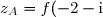) et
et =-\text i) .
.) , représentative dans le repère
, représentative dans le repère  de
de  vers
vers =(x+1)\ln(x^2+2x+1),&\text{si }x\neq-1\\g(-1)=0\end{matrix}\right.)
 est la fonction
  :
:\ \cos x-\sin x \quad B)\ x\cos x \quad C)\ \cos x+\sin x \quad D)\ -x\cos x)
) au plan
au plan  : 2x-y+3z+5=0) est :
est :\ \sqrt6 \quad B)\ \sqrt{14} \quad C)\ \dfrac{6\sqrt{14}}{7} \quad D)\ \dfrac{6\sqrt7}{7})
e^{-x}=)
\ -\infty \quad B)\ +\infty \quad C)\ 0 \quad D)\ 4)
) . Soit
. Soit  la similitude directe de centre
 ) , de rapport
, de rapport  et d'angle de mesure
  . L'écriture complexe de
 \ z'=(1+\text i\sqrt3)z+\sqrt3-\text i\sqrt3 \quad B)\ z'=(\sqrt3+\text i)z+\sqrt3-\text i\sqrt3 \quad C)\ z'=(1+\text i\sqrt3)z-\sqrt3+\text i\sqrt3 \quad D)\ z'=(1-\text i\sqrt3)z+\sqrt3-\text i\sqrt3)
 la fonction numérique définie par
 =\left\lbrace\begin{matrix}\dfrac{2\sqrt x-2}{x-1}&\text{si }x\in[0;1[\\ax^2+x+a-6&\text{si }x\in[1;+\infty[\end{matrix}\right.) où
où  est un nombre réel.
 si et seulement si :
\ a=-2 \quad B)\ a=0 \quad C)\ a=3 \quad D)\ a=1)
 la suite géométrique de premier terme
  et de raison
  .
. est égal à :
\ \text e^{\frac{n(n+1)}{2}} \quad B)\ \text e^{n(n+1)} \quad C)\ \text e^{\frac{n(n-1)}{2}} \quad D)\ \text e^{n(n-1)})
 .
Une primitive de
.
Une primitive de 
 sur
sur  ,
, =\ldots b\ldots) .
Une similitude plane directe est une transformation du plan dans lui-même,
qui multiplie les
.
Une similitude plane directe est une transformation du plan dans lui-même,
qui multiplie les  par un nombre réel strictement positif
  .
Le nombre réel positif
.
Le nombre réel positif  de la similitude.
Si le plan complexe est rapporté à un repère orthonormé alors l'écriture complexe d'une similitude plane
directe
de la similitude.
Si le plan complexe est rapporté à un repère orthonormé alors l'écriture complexe d'une similitude plane
directe  .
Si
.
Si  alors
alors  .
Si
.
Si  .
. boules blanches,
  boules rouges.
 boules de cette urne.
 indiquant le nombre de boules noires parmi les
  :~y'=y) où
où  est une fonction dérivable de la variable réelle
  .
.) .
. :~y'=y-\cos(x)-3\sin(x)) où
où  définie sur
 =2\cos(x)+\sin(x)) .
.) .
. est solution de
 =0) .
.![\displaystyle\int_0^{\frac{\pi}{2}}\left[-2e^x+\sin(x)+2\cos(x)\right]\,\text dx](https://latex.ilemaths.net/latex-0.tex?\displaystyle\int_0^{\frac{\pi}{2}}\left[-2e^x+\sin(x)+2\cos(x)\right]\,\text dx) .
.
 forum de terminale