Bac S Obligatoire et Spécialité Antilles Guyane 2018
Partager :
5 points
exercice 1 - Commun à tous les candidats
Partie A
1. Arbre pondéré traduisant la situation :
2. Nous devons déterminer
D'où la probabilité que l'arbre abattu soit un chêne vendu à un habitant de la commune est égale à 0,1377.
3. Nous devons déterminer
En utilisant la formule des probabilités totales, nous avons :
D'où la probabilité que l'arbre abattu soit vendu à un habitant de la commune est égale à 0,5877
4. Nous devons déterminer
Par conséquent, la probabilité qu'un arbre abattu vendu à un habitant de la commune soit un sapin est environ égale à 0,681 (arrondie à 10-3).
Partie B
Le nombre d'arbres sur un hectare de cette forêt peut être modélisé par une variable aléatoire X suivant une loi normale d'espérance = 4000 et d'écart-type = 300.
1. Par la calculatrice, nous obtenons
D'où la probabilité qu'il y ait entre 3400 et 4600 arbres sur un hectare donné de cette forêt est environ égale à 0,954 (arrondie à 10-3).
Nous pouvions trouver ce résultat par la propriété suivante de la loi normale :
En effet, nous obtenons alors :
2. Nous devons déterminer
Nous savons que , soit que
Par conséquent, la probabilité qu'il y ait plus de 4500 arbres sur un hectare donné de cette forêt est environ égale à 0,048 (arrondie à 10-3).
Partie C
Déterminons un intervalle de fluctuation asymptotique I200 au seuil de 95 % de la proportion de sapins dans cette forêt communale.
Les conditions d'utilisation de l'intervalle de fluctuation sont remplies.
En effet,
Donc un intervalle de fluctuation asymptotique I200 au seuil de 95% est :
La fréquence observée est
Nous remarquons que
Par conséquent, au risque de se tromper de 5%, l'affirmation de l'exploitant ne doit pas être remise en question.
5 points
exercice 2 - Commun à tous les candidats
1. Nous utiliserons le théorème suivant : Si deux plans sont parallèles, tout plan sécant les coupe suivant des droites parallèles.
Les plans (FGH) et (BCD) sont parallèles.
Le plan (SLM) coupe (FGH) et (BCD) suivant les droites (LM) et (BD).
En utilisant le théorème ci-dessus, les droites (LM) et (BD) sont parallèles.
2. Soit le repère orthonormé
Sachant que les longueurs des arêtes du cube sont égales à 6 mètres, nous obtenons E(0 ; 0 ; 6) et F(6 ; 0 ; 6).
D'où, les coordonnées du point L sont (2 ; 0 ; 6).
3. a. Déterminons une représentation paramétrique de la droite (BL).
La droite (BL) est dirigée par le vecteur
La droite (BL) passe par le point
D'où une représentation paramétrique de la droite (BL) est donnée par :
soit
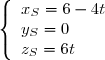
3. b. Le point S appartient à la droite (AK).
Ses coordonnées sont donc de la forme (0 ; 0 ; zS ), soit xS = 0 et yS = 0.
Le point S appartient également à la droite (BL).
Il existe alors un réel t tel que
Remplaçons t par dans la relation zS = 6t .
Par conséquent, les coordonnées du point S sont (0 ; 0 ; 9).
Puisque le vecteur est orthogonal aux deux vecteurs manifestement non colinéaires et , nous en déduisons que le vecteur est normal au plan (BDL).
4. b.
Nous savons que tout plan de vecteur normal admet une équation cartésienne de la forme ax + by + cz + d = 0.
Puisque le vecteur est normal au plan (BDL), une équation cartésienne du plan (BDL) est de la forme 3x + 3y + 2z + d = 0.
Or le point B(6 ; 0 ; 0) appartient au plan (BDL). Ses coordonnées vérifient l'équation du plan.
D'où , soit 18 + d = 0 soit d = -18.
Par conséquent, une équation cartésienne du plan (BDL) est :
4. c. Le point M est le point commun à la droite (EH) et au plan (BDL).
Les coordonnées de ce point sont les solutions du système composé par les équations de la droite (EH) et du plan (BDL),
soit du système :
D'où les coordonnées du point M sont
5. Calculons le volume du tétraèdre SELM :
Le triangle ELM est rectangle en E.
Nous en déduisons que
Par conséquent,
6. Dans le triangle SEL rectangle en E, nous avons :
Puisque la mesure de l'angle est comprise entre 55° et 60°, la contrainte d'angle est respectée.
5 points
exercice 3 - Commun à tous les candidats
Partie A - Etude de la fonction f
1. Pour tout x,
2. Limite de f en + :
En utilisant le théorème d'encadrement, nous obtenons :
4. a) Puisque pour tout x et a fortiori pour tout x [- ; ], e-x > 0,
nous en déduisons que le signe de f' (x ) sera le signe de 2cos x - 1.
Résolvons d'abord l'équation dans l'intervalle
4. b. Variations de f sur l'intervalle [- ; ]
Donc f est décroissante sur l'intervalle f est croissante sur l'intervalle f est décroissante sur l'intervalle
Partie B - Aire du logo
1. Etudions le signe de f (x ) - g (x ).
Dès lors, pour tout x réel, f (x ) - g (x ) 0.
Par conséquent, la courbe Cf est au-dessus de la courbe Cg sur .
2. a. Représentation graphique du domaine D .
2. b. Nous avons montré dans la question 1. que la courbe Cf est au-dessus de la courbe Cg sur .
Il en est évidemment de même sur l'intervalle
D'où l'aire du domaine D , en unité d'aire, se calcule par
Pusque l'unité graphique est de 2 centimètres,
Nous obtenons ainsi
5 points
exercice 4 - Candidats n'ayant pas suivi l'enseignement de spécialité
1. Le 1er juin 2017, le nombre de cétacés est
Entre le 1er juin et le 31 octobre 2017, 80 cétacés arrivent dans la réserve marine.
Donc le 31 octobre 2017, il y a 3 000 + 80 = 3 080 cétacés.
Entre le 1er novembre 2017 et le 31 mai 2018, la réserve subit une baisse de 5% de son effectif par rapport à celui du 31 octobre qui précède, soit une baisse de 5% de 3080 cétacés.
Par conséquent, le 1er juin 2018, le nombre de cétacés est
2. Le 1er juin 2017 + n , le nombre de cétacés est
Entre le 1er juin et le 31 octobre 2017 + n , 80 cétacés arrivent dans la réserve marine.
Donc le 31 octobre 2017 + n , il y a cétacés.
Entre le 1er novembre 2017 + n et le 31 mai 2017 + (n + 1), la réserve subit une baisse de 5% de son effectif par rapport à celui du 31 octobre qui précède, soit une baisse de 5% de cétacés.
Par conséquent,
le 1er juin 2017 + (n + 1), le nombre de cétacés est
soit
3. La formule à entrer dans la cellule C2 est
4. a. Montrons par récurrence que pour tout entier naturel n ,
Initialisation : Montrons que la propriété est vraie pour n = 0.
Nous savons que
La propriété est donc démontrée pour n = 0.
Hérédité : Supposons que pour un entier naturel n fixé la propriété soit vraie au rang n et montrons qu'elle est encore vraie au rang n + 1.
Supposons donc que pour un entier naturel n fixé,
Montrons que nous avons
En effet, nous savons par la question 2. que
Dès lors,
L'hérédité est donc démontrée.
Puisque l'initialisation et l'hérédité sont vraies, nous avons démontré par récurrence que pour tout entier naturel n ,
Or nous savons par la question précédente que .
Par conséquent, la suite (un ) est décroissante.
4. c) La suite (un ) étant décroissante et bornée inférieurement par 1520, nous en déduisons que cette suite (un ) est convergente.
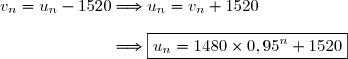
5. Soit
D'où la suite (vn ) est une suite géométrique de raison q = 0,95 et dont le premier terme est
5. b)
5. c)
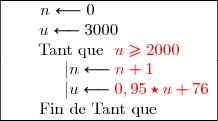
6. Algorithme complété :
7. Nous savons que la limite de la suite (un ) est égale à 1520.
Or le classement de la zone en "réserve marine" ne sera pas reconduit si le nombre de cétacés de la réserve devient inférieur à 2000.
Puisque 1520 < 2000, la réserve marine fermera un jour.
Nous déterminerons l'année de fermeture en résolvant dans , l'inéquation un < 2000.
Puisque n est un nombre entier, la plus petite valeur de n vérifiant l'inéquation est donc n = 22.
2017 + 22 = 2039.
Par conséquent, la réserve marine fermera en 2039.
5 points
exercice 4 - Candidats ayant suivi l'enseignement de spécialité
1. Chaque année, 65% des possesseurs de la carte de pêche libre achètent de nouveau une carte de pêche libre l'année suivante
et 45% des possesseurs de la carte de pêche avec quota achètent une carte de pêche libre l'année suivante.
Nous avons donc la relation suivante :
On suppose dans l'énoncé que le nombre total de pêcheurs reste constant d'année en année.
Donc a contrario, chaque année, 35% des possesseurs de la carte de pêche libre achètent une carte de pêche avec quota l'année suivante
et 55% des possesseurs de la carte de pêche avec quota achètent de nouveau une carte de pêche avec quota l'année suivante.
Nous avons donc la relation suivante :
2. Nous devons déterminer la valeur de q 2.
Nous en déduisons que q 2 = 0,444.
Par conséquent, la proportion de pêcheurs achetant une carte de pêche avec quota en 2019 est de 44,4%.
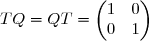
3. a. Puisque , la matrice Q est inversible.
De plus, la matrice inverse de Q est
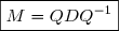
3. b. Par le logiciel, nous savons que D = TMQ.
Par conséquent,
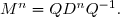
Montrons par récurrence que pour tout entier naturel n non nul,
Initialisation : Montrons que la propriété est vraie pour n = 1.
Montrons donc que
La propriété est donc démontrée pour n = 1.
Hérédité : Supposons que pour un entier naturel n non nul fixé la propriété soit vraie au rang n et montrons qu'elle est encore vraie au rang n + 1.
Supposons donc que pour un entier naturel n non nul fixé,
Montrons que nous avons
En effet,
L'hérédité est donc démontrée.
Puisque l'initialisation et l'hérédité sont vraies, nous avons démontré par récurrence que pour tout entier naturel n non nul,
4. a. Nous avons montré dans la question 1. que pour tout entier n , .
Dès lors, la suite est une suite géométrique de raison M et dont le premier terme est .
Par conséquent, l'écriture explicite du terme général de cette suite est Pn = MnP0 .
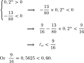
5. Pour tout entier naturel n ,
Par conséquent, la proportion de pêcheurs achetant la carte de pêche libre ne dépassera pas 60%.
Publié par malou
le
ceci n'est qu'un extrait
Pour visualiser la totalité des cours vous devez vous inscrire / connecter (GRATUIT) Inscription Gratuitese connecter
Merci à Hiphigenie / malou pour avoir contribué à l'élaboration de cette fiche
Désolé, votre version d'Internet Explorer est plus que périmée ! Merci de le mettre à jour ou de télécharger Firefox ou Google Chrome pour utiliser le site. Votre ordinateur vous remerciera !


.)
=P(C)\times _{C}(H)\\\phantom{P(C\cap H)}=0,3\times0,459\\\phantom{P(C\cap H)}=0,1377\\\\\Longrightarrow\boxed{P(C\cap H)=0,1377})
.)
= P(C\cap H)+P(S\cap H)+P(E\cap H) \\\phantom{P(H)}=P(C)\times P_{C}(H)+P(S)\times P_{S}(H)+P(E)\times P_{E}(H) \\\phantom{P(H)}=0,3\times0,459+0,5\times0,8+0,2\times0,25 \\\phantom{P(H)}=0,1377+0,4+0,05 \\\phantom{P(H)}=0,5877 \\\\\Longrightarrow\boxed{P(H)=0,5877})
)
=\dfrac{P(S\cap H)}{P(H)} \\\\\phantom{P_H(S)}=\dfrac{P(S)\times P_S(H)}{0,5877} \\\\\phantom{P_H(S)}=\dfrac{0,5\times 0,8}{0,5877} \\\\\phantom{P_H(S)}\approx 0,6806193636)
 = 4000 et d'écart-type
  = 300.
\approx0,95449973)
\approx0,954.)
=P(4000-600\le X\le4000+600)\\\phantom{P(3400\le X\le4600)}=P(4000-2\times300\le X\le4000+2\times300)\\\phantom{P(81,6\le X\le82,4)}=P(\mu-\sigma\le X\le\mu+\sigma)\\\phantom{P(81,6\le X\le82,4)}\approx\boxed{0,954})
.)
=0,5) , soit que
, soit que =0,5)
=0,5\Longleftrightarrow P(4000\le X\le4500)+P(X>4500)=0,5 \\\phantom{\text{Dès lors, }\ P(X\ge4000)=0,5}\Longleftrightarrow P(X>4500)=0,5-P(4000\le X\le4500) \\\phantom{\text{Dès lors, }\ P(X\ge4000)=0,5}\Longrightarrow P(X>4500)\approx0,5-0,45220964 \\\phantom{\text{Dès lors, }\ P(X\ge4000)=0,5}\Longrightarrow P(X>4500)\approx0,04779036)
= 200\times(1-0,5)= 200\times0,5=100\ge5 \end{array})
![I_{200}=\left[0,5-1,96\sqrt{\dfrac{0,5 (1-0,5)}{200}};0,5+1,96\sqrt{\dfrac{0,5 (1-0,5)}{200}}\right]\\\\\Longrightarrow I_{200}\approx[0,431;0,569]](https://latex.ilemaths.net/latex-0.tex? I_{200}=\left[0,5-1,96\sqrt{\dfrac{0,5 (1-0,5)}{200}};0,5+1,96\sqrt{\dfrac{0,5 (1-0,5)}{200}}\right]\\\\\Longrightarrow I_{200}\approx[0,431;0,569])

.)
\\ E(0;0;6)\end{matrix}\right.\Longrightarrow\overrightarrow{FE}\begin{pmatrix}0-6\\0-0\\6-6\end{pmatrix}\Longrightarrow\overrightarrow{FE}\begin{pmatrix}-6\\0\\0\end{pmatrix})
\\ L(x_L;y_L;z_L)\end{matrix}\right.\Longrightarrow\overrightarrow{FL}\begin{pmatrix}x_L-6\\y_L-0\\z_L-6\end{pmatrix}\Longrightarrow\overrightarrow{FL}\begin{pmatrix}x_L-6\\y_L\\z_L-6\end{pmatrix})
\\\\\dfrac{2}{3}\times0\\\\\dfrac{2}{3}\times0\end{pmatrix} \\\\\\\phantom{\overrightarrow{FL}=\dfrac{2}{3}\overrightarrow{FE}}\Longrightarrow\begin{pmatrix}x_L-6\\y_L\\z_L-6\end{pmatrix}=\begin{pmatrix}-4\\0\\0\end{pmatrix} \ \ \ \Longrightarrow\left\lbrace\begin{matrix}x_L-6=-4\\y_L=0\\z_L-6=0\end{matrix}\right. \ \ \ \Longrightarrow\boxed{\left\lbrace\begin{matrix}x_L=2\\y_L=0\\z_L=6\end{matrix}\right.})

\\L(2;0;6)\end{array}\Longrightarrow\overrightarrow{BL}\begin{pmatrix}2-6\\0-0 \\6-0\end{pmatrix}\Longrightarrow\boxed{\overrightarrow{BL}\begin{pmatrix}{\red{-4}}\\ {\red{0}}\\ {\red{6}}\end{pmatrix}})
.)
)
:\left\lbrace\begin{array}l x=6-4t\\y=0\\z=6t \end{array}\ \ \ (t\in\mathbb{R})})

 dans la relation z S = 6t .
\\ D(0;6;0)\end{matrix}\right.\Longrightarrow\overrightarrow{BD}\begin{pmatrix}0-6\\6-0\\0-0\end{pmatrix}\Longrightarrow\overrightarrow{BD}\begin{pmatrix}-6\\6\\0\end{pmatrix})
+3\times6+2\times0\\=-18+18+0\ \ \ \ \ \\=0\ \ \ \ \ \ \ \ \ \ \ \ \ \ \ \ \ \ \ \ \ \\\\\Longrightarrow\boxed{\overrightarrow{n}\perp\overrightarrow{BD}}\ \ \ \ \ \ \ \ \ \ \ \ \ \ \ \ \ \ \ \ \ \end{matrix})
+3\times0+2\times6\\=-12+0+12\ \ \ \ \ \\=0\ \ \ \ \ \ \ \ \ \ \ \ \ \ \ \ \ \ \ \ \ \\\\\Longrightarrow\boxed{\overrightarrow{n}\perp\overrightarrow{BL}}\ \ \ \ \ \ \ \ \ \ \ \ \ \ \ \ \ \ \ \ \ \end{matrix})
 est orthogonal aux deux vecteurs manifestement non colinéaires
  et
et  , nous en déduisons que le vecteur
  admet une équation cartésienne de la
  est normal au plan (BDL), une équation cartésienne du plan (BDL) est de la
  , soit 18 + d = 0 soit d = -18.


}.)


\\ L(2;0;6)\end{matrix}\right.\Longrightarrow\overrightarrow{EL}\begin{pmatrix}2-0\\0-0\\6-6\end{pmatrix}\Longrightarrow\overrightarrow{EL}\begin{pmatrix}2\\0\\0\end{pmatrix}\Longrightarrow EL=2 \\\\\phantom{\text{Or }}\left\lbrace\begin{matrix}E(0;0;6)\\ M(0;2;6)\end{matrix}\right.\Longrightarrow\overrightarrow{EM}\begin{pmatrix}0-0\\2-0\\6-6\end{pmatrix}\Longrightarrow\overrightarrow{EM}\begin{pmatrix}0\\2\\0\end{pmatrix}\Longrightarrow EM=2 \\\\\text{D'où }\ \mathscr{A}_{ELM}=\dfrac{1}{2}\times 2\times 2 \\\\\phantom{\text{D'où }}\ \boxed{\mathscr{A}_{ELM}=2})
\\ S(0;0;9)\end{matrix}\right.\Longrightarrow\overrightarrow{ES}\begin{pmatrix}0-0\\0-0\\9-6\end{pmatrix}\Longrightarrow\overrightarrow{ES}\begin{pmatrix}0\\0\\3\end{pmatrix}\Longrightarrow ES=3)
=\dfrac{ES}{EL}\Longrightarrow\tan(\widehat{SLE})=\dfrac{3}{2}\\\\\text{D'où }\ \widehat{SLE}=\arctan(\dfrac{3}{2}) \\\\\phantom{\text{D'où }\ }\boxed{\widehat{SLE}\approx56,3^{\text{o}}})
 est comprise entre 55° et 60°, la contrainte d'angle est respectée.
 ,
, \times \text{e}^{-x}\le3\times \text{e}^{-x}\ \ \ \ \ \ \ (\text{car }\text{e}^{-x}>0) \\\\\phantom{\text{Donc }\ }-\text{e}^{-x}\le\text{e}^{-x}(-\cos x +\sin x +1)\le3\text{e}^{-x} \\\\\Longrightarrow\boxed{-\text{e}^{-x}\le f(x)\le3\text{e}^{-x}})
 :
: =-\infty\\\\\lim\limits_{X\to-\infty}\text{e}^X =0\end{matrix}\right.\ \ \Longrightarrow\lim\limits_{x\to+\infty}\text{e}^{-x}=0\ \ \Longrightarrow\left\lbrace\begin{matrix}\lim\limits_{x\to+\infty}-\text{e}^{-x}=0\\\\\lim\limits_{x\to+\infty}3\text{e}^{-x}=0\end{matrix}\right.)
\le3\text{e}^{-x}\\\\\lim\limits_{x\to+\infty}(-\text{e}^{-x})=\lim\limits_{x\to+\infty}3\text{e}^{-x}=0\end{matrix}\right.\ \ \Longrightarrow\boxed{\lim\limits_{x\to+\infty}f(x)=0})
![{\red{\text{3. }}}\text{Pour tout }x\in\mathbb{R},\ \ f'(x)=[\text{e}^{-x}(-\cos x +\sin x +1)]'\\\\\phantom{{\red{\text{3. }}}\text{Pour tout }x\in\mathbb{R},\ \ f'(x)}=(\text{e}^{-x})'\times(-\cos x +\sin x +1)+\text{e}^{-x}\times(-\cos x +\sin x +1)' \\\\\phantom{{\red{\text{3. }}}\text{Pour tout }x\in\mathbb{R},\ \ f'(x)}=(-\text{e}^{-x})\times(-\cos x +\sin x +1)+\text{e}^{-x}\times(\sin x +\cos x +0) \\\\\phantom{{\red{\text{3. }}}\text{Pour tout }x\in\mathbb{R},\ \ f'(x)}=-\text{e}^{-x}(-\cos x +\sin x +1)+\text{e}^{-x}(\sin x +\cos x) \\\\\phantom{{\red{\text{3. }}}\text{Pour tout }x\in\mathbb{R},\ \ f'(x)}=\text{e}^{-x}[-(-\cos x +\sin x +1)+(\sin x +\cos x)] \\\\\phantom{{\red{\text{3. }}}\text{Pour tout }x\in\mathbb{R},\ \ f'(x)}=\text{e}^{-x}(\cos x -\sin x -1+\sin x +\cos x) \\\\\phantom{{\red{\text{3. }}}\text{Pour tout }x\in\mathbb{R},\ \ f'(x)}=\text{e}^{-x}(2\cos x-1) \\\\\Longrightarrow\boxed{f'(x)=\text{e}^{-x}(2\cos x -1)}](https://latex.ilemaths.net/latex-0.tex?{\red{\text{3. }}}\text{Pour tout }x\in\mathbb{R},\ \ f'(x)=[\text{e}^{-x}(-\cos x +\sin x +1)]'\\\\\phantom{{\red{\text{3. }}}\text{Pour tout }x\in\mathbb{R},\ \ f'(x)}=(\text{e}^{-x})'\times(-\cos x +\sin x +1)+\text{e}^{-x}\times(-\cos x +\sin x +1)' \\\\\phantom{{\red{\text{3. }}}\text{Pour tout }x\in\mathbb{R},\ \ f'(x)}=(-\text{e}^{-x})\times(-\cos x +\sin x +1)+\text{e}^{-x}\times(\sin x +\cos x +0) \\\\\phantom{{\red{\text{3. }}}\text{Pour tout }x\in\mathbb{R},\ \ f'(x)}=-\text{e}^{-x}(-\cos x +\sin x +1)+\text{e}^{-x}(\sin x +\cos x) \\\\\phantom{{\red{\text{3. }}}\text{Pour tout }x\in\mathbb{R},\ \ f'(x)}=\text{e}^{-x}[-(-\cos x +\sin x +1)+(\sin x +\cos x)] \\\\\phantom{{\red{\text{3. }}}\text{Pour tout }x\in\mathbb{R},\ \ f'(x)}=\text{e}^{-x}(\cos x -\sin x -1+\sin x +\cos x) \\\\\phantom{{\red{\text{3. }}}\text{Pour tout }x\in\mathbb{R},\ \ f'(x)}=\text{e}^{-x}(2\cos x-1) \\\\\Longrightarrow\boxed{f'(x)=\text{e}^{-x}(2\cos x -1)})
 ;
;  dans l'intervalle
 ![[-\pi;\pi].](https://latex.ilemaths.net/latex-0.tex?[-\pi;\pi].)
![\text{Si }\ x\in[-\pi;\pi], \ \text{alors }\ \ 2\cos x-1=0\Longleftrightarrow2\cos x=1\\\phantom{\text{Si }\ x\in[-\pi;\pi], \ \text{alors }\ \ 2\cos x-1=0}\Longleftrightarrow\cos x=\dfrac{1}{2}\\\phantom{\text{Si }\ x\in[-\pi;\pi], \ \text{alors }\ \ 2\cos x-1=0}\Longleftrightarrow x=\dfrac{\pi}{3}\ \ \text{ou}\ \ x=-\dfrac{\pi}{3}](https://latex.ilemaths.net/latex-0.tex?\text{Si }\ x\in[-\pi;\pi], \ \text{alors }\ \ 2\cos x-1=0\Longleftrightarrow2\cos x=1\\\phantom{\text{Si }\ x\in[-\pi;\pi], \ \text{alors }\ \ 2\cos x-1=0}\Longleftrightarrow\cos x=\dfrac{1}{2}\\\phantom{\text{Si }\ x\in[-\pi;\pi], \ \text{alors }\ \ 2\cos x-1=0}\Longleftrightarrow x=\dfrac{\pi}{3}\ \ \text{ou}\ \ x=-\dfrac{\pi}{3})
![\text{D'où }\ f'(x)\le0\Longleftrightarrow x\in[-\pi;-\dfrac{\pi}{3}]\ \cup\ [\dfrac{\pi}{3};\pi] \\\\\phantom{\text{D'où }\ }f'(x)\ge0\Longleftrightarrow x\in\ [-\dfrac{\pi}{3};\dfrac{\pi}{3}]](https://latex.ilemaths.net/latex-0.tex?\text{D'où }\ f'(x)\le0\Longleftrightarrow x\in[-\pi;-\dfrac{\pi}{3}]\ \cup\ [\dfrac{\pi}{3};\pi] \\\\\phantom{\text{D'où }\ }f'(x)\ge0\Longleftrightarrow x\in\ [-\dfrac{\pi}{3};\dfrac{\pi}{3}])
&&-&0&+&0&-&\\\hline &2e^{\pi}\approx46,281&&&&\approx0,4793&&&f(x)&&\searrow&&\nearrow&&\searrow&\\&&&\approx-1,0430&&&&2e^{-\pi}\approx0,0864\\\hline \end{array})
![[-\pi;-\dfrac{\pi}{3}]](https://latex.ilemaths.net/latex-0.tex?[-\pi;-\dfrac{\pi}{3}])
![[-\dfrac{\pi}{3};\dfrac{\pi}{3}]](https://latex.ilemaths.net/latex-0.tex?[-\dfrac{\pi}{3};\dfrac{\pi}{3}])
![[\dfrac{\pi}{3};\pi]](https://latex.ilemaths.net/latex-0.tex?[\dfrac{\pi}{3};\pi])
-g(x)=\text{e}^{-x}(-\cos x +\sin x +1)-(-\text{e}^{-x}\cos x) \\\phantom{f(x)-g(x)}=\text{e}^{-x}(-\cos x +\sin x +1)+\text{e}^{-x}\cos x \\\phantom{f(x)-g(x)}=\text{e}^{-x}(-\cos x +\sin x +1+\cos x) \\\phantom{f(x)-g(x)}=\text{e}^{-x}(\sin x +1) \\\\\Longrightarrow\boxed{f(x)-g(x)=\text{e}^{-x}(\sin x +1)}\\\\\text{Or pour tout }x\text{ réel, }\ \left\lbrace\begin{matrix}\text{e}^{-x}>0\\\sin x\ge-1\end{matrix}\right.\Longrightarrow\left\lbrace\begin{matrix}\text{e}^{-x}>0\\\sin x+1\ge0\end{matrix}\right.)
 0.
0.
![[-\dfrac{\pi}{2};\dfrac{3\pi}{2}].](https://latex.ilemaths.net/latex-0.tex?[-\dfrac{\pi}{2};\dfrac{3\pi}{2}].)
![\mathscr{A}=\int\limits_{-\frac{\pi}{2}}^{\frac{3\pi}{2}}(f(x)-g(x))\,dx \\\\ \phantom{ aa} =\left[H(x) \right]\limits_{-\frac{\pi}{2}}^{\frac{3\pi}{2}} \\\\ \phantom{ aa} =H(\dfrac{3\pi}{2})-H(-\dfrac{\pi}{2}) \\\\\text{Or }\ H(\dfrac{3\pi}{2})=(-\dfrac{\cos\dfrac{3\pi}{2}}{2}-\dfrac{\sin\dfrac{3\pi}{2}}{2}-1)\text{e}^{-\frac{3\pi}{2}} =(0-\dfrac{-1}{2}-1)\text{e}^{-\frac{3\pi}{2}}=-\dfrac{1}{2}\text{e}^{-\frac{3\pi}{2}} \\\\\phantom{\text{Or }\ }H(-\dfrac{\pi}{2})=(-\dfrac{\cos(-\dfrac{\pi}{2})}{2}-\dfrac{\sin(-\dfrac{\pi}{2})}{2}-1)\text{e}^{\frac{\pi}{2}} =(0-\dfrac{-1}{2}-1)\text{e}^{\frac{\pi}{2}}=-\dfrac{1}{2}\text{e}^{\frac{\pi}{2}} \\\\\text{D'où }\ \mathscr{A}=-\dfrac{1}{2}\text{e}^{-\frac{3\pi}{2}}-(-\dfrac{1}{2}\text{e}^{\frac{\pi}{2}})](https://latex.ilemaths.net/latex-0.tex?\mathscr{A}=\int\limits_{-\frac{\pi}{2}}^{\frac{3\pi}{2}}(f(x)-g(x))\,dx \\\\ \phantom{ aa} =\left[H(x) \right]\limits_{-\frac{\pi}{2}}^{\frac{3\pi}{2}} \\\\ \phantom{ aa} =H(\dfrac{3\pi}{2})-H(-\dfrac{\pi}{2}) \\\\\text{Or }\ H(\dfrac{3\pi}{2})=(-\dfrac{\cos\dfrac{3\pi}{2}}{2}-\dfrac{\sin\dfrac{3\pi}{2}}{2}-1)\text{e}^{-\frac{3\pi}{2}} =(0-\dfrac{-1}{2}-1)\text{e}^{-\frac{3\pi}{2}}=-\dfrac{1}{2}\text{e}^{-\frac{3\pi}{2}} \\\\\phantom{\text{Or }\ }H(-\dfrac{\pi}{2})=(-\dfrac{\cos(-\dfrac{\pi}{2})}{2}-\dfrac{\sin(-\dfrac{\pi}{2})}{2}-1)\text{e}^{\frac{\pi}{2}} =(0-\dfrac{-1}{2}-1)\text{e}^{\frac{\pi}{2}}=-\dfrac{1}{2}\text{e}^{\frac{\pi}{2}} \\\\\text{D'où }\ \mathscr{A}=-\dfrac{1}{2}\text{e}^{-\frac{3\pi}{2}}-(-\dfrac{1}{2}\text{e}^{\frac{\pi}{2}}))

\times4\ \text{cm}^2\approx9,60\ \text{cm}^2})


) cétacés.
cétacés. = 0,05\times(u_n+80) \\\phantom{5\%\ \text{de }(u_n+80) }=0,05\times u_n+0,05\times80 \\\phantom{5\%\ \text{de }(u_n+80) }=0,05u_n+4)
-(0,05u_n+4)=u_n-0,05u_n+80-4)


} \\\\\phantom{u_{n+1}=0,95u_n+76}\Longrightarrow\boxed{u_{n+1}\ge1520}\ \ \ \ \ (\text{car }\ 0,95\times1520+76=1520))
 }}}\ u_{n+1}-u_n=(0,95u_n+76)-u_n\\\phantom{{\red{\text{3. b) }}}\ p_{n+1}-p_n}=0,95u_n-u_n+76 \\\phantom{{\red{\text{3. b) }}}\ p_{n+1}-p_n}=-0,05u_n+76 \\\\\Longrightarrow\boxed{ u_{n+1}-u_n=-0,05u_n+76}\ \ \ {\red{(1)}})
 .
.\times u_n\le(-0,05)\times1520 \\\phantom{u_n>1520}\Longrightarrow-0,05u_n\le-76 \\\phantom{u_n>1520}\Longrightarrow\boxed{-0,05u_n+76\le0}\ \ \ {\red{(2)}} \\\\\\\ \ \ {\red{(1)}}\ \text{et}\ {\red{(2)}}\Longrightarrow\boxed{ u_{n+1}-u_n\le0})
)
 }}}\ v_{n+1}=u_{n+1}-1520\\\phantom{{\red{\text{4. a) }}}\ v_{n+1}}=(0,95u_n+76)-1520 \\\phantom{{\red{\text{4. a) }}}\ v_{n+1}}=0,95u_n-1444 \\\phantom{{\red{\text{4. a) }}}\ v_{n+1}}=0,95u_n-0,95\times1520 \\\phantom{{\red{\text{4. a) }}}\ v_{n+1}}=0,95(u_n-1520) \\\phantom{{\red{\text{4. a) }}}\ v_{n+1}}=0,95v_n \\\\\Longrightarrow\boxed{v_{n+1}=0,95v_n})


)
![\Longrightarrow\lim\limits_{n\to+\infty}u_n=\lim\limits_{n\to+\infty}[1480\times0,95^n+1520]\\\\\phantom{\Longrightarrow\lim\limits_{n\to+\infty}p_n}=1480\times\lim\limits_{n\to+\infty}(0,95^{n})+1520 \\\\\phantom{\Longrightarrow\lim\limits_{n\to+\infty}p_n}=1480\times0+1520 \\\\\phantom{\Longrightarrow\lim\limits_{n\to+\infty}p_n}=1520 \\\\\Longrightarrow\boxed{\lim\limits_{n\to+\infty}u_n=1520}](https://latex.ilemaths.net/latex-0.tex?\Longrightarrow\lim\limits_{n\to+\infty}u_n=\lim\limits_{n\to+\infty}[1480\times0,95^n+1520]\\\\\phantom{\Longrightarrow\lim\limits_{n\to+\infty}p_n}=1480\times\lim\limits_{n\to+\infty}(0,95^{n})+1520 \\\\\phantom{\Longrightarrow\lim\limits_{n\to+\infty}p_n}=1480\times0+1520 \\\\\phantom{\Longrightarrow\lim\limits_{n\to+\infty}p_n}=1520 \\\\\Longrightarrow\boxed{\lim\limits_{n\to+\infty}u_n=1520})
 , l'inéquation un < 2000.
<\ln(\dfrac{12}{37}) \\\\\phantom{u_n<2000}\Longleftrightarrow n\times\ln(0,95)<\ln(\dfrac{12}{37}) \\\\\phantom{u_n<2000}\Longleftrightarrow n>\dfrac{\ln(\dfrac{12}{37})}{\ln(0,95)}\ \ \ \ \text{(Changement de sens de l'inégalité car }\ln(0,95)<0) \\\\\text{Or }\ \dfrac{\ln(\dfrac{12}{37})}{\ln(0,95)}\approx21,95)


 , la matrice Q est inversible.
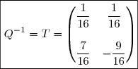
M(QQ^{-1})}\\\\\text{Or, par le logiciel, }\ QT=\begin{pmatrix}1&0\\0&1\end{pmatrix}=I\\\text{et }\ QQ^{-1}=\begin{pmatrix}1&0\\0&1\end{pmatrix}=I \\\\\text{Donc }\ QDQ^{-1}=IMI=M)
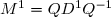
 \\\phantom{M^1}=QD^1Q^{-1} \\\\\Longrightarrow\boxed{M^1=QD^1Q^{-1}})
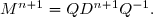
DQ^{-1} \\\\\phantom{M^{n+1}}=QD^nIDQ^{-1} \\\\\phantom{M^{n+1}}=QD^nDQ^{-1} \\\\\phantom{M^{n+1}}=QD^{n+1}Q^{-1}\\\\\Longrightarrow\boxed{M^{n+1}=QD^{n+1}Q^{-1}})
 .
._{n\in\mathbb{N}}) est une suite géométrique de raison M et dont le premier terme est
est une suite géométrique de raison M et dont le premier terme est  .
.![{\red{\text{4.b.}}}\ \ P_n=M^nP_0\Longleftrightarrow\begin{pmatrix}\ell_n\\q_n\end{pmatrix}=\dfrac{1}{16}\begin{pmatrix}9+7\times0,2^n &9-9\times0,2^n \\7-7\times0,2^n & 7+9\times0,2^n\end{pmatrix}\begin{pmatrix}0,4\\0;6\end{pmatrix} \\\\\Longrightarrow\ell_n=\dfrac{1}{16}[(9+7\times0,2^n)\times0,4+(9-9\times0,2^n )\times0,6] \\\\\phantom{\Longrightarrow\ell_n}=\dfrac{1}{16}[3,6+2,8\times0,2^n+5,4-5,4\times0,2^n ] \\\\\phantom{\Longrightarrow\ell_n}=\dfrac{1}{16}(9-2,6\times0,2^n) \\\\\phantom{\Longrightarrow\ell_n}=\dfrac{1}{16}(9-\dfrac{13}{5}\times0,2^n) \\\\\phantom{\Longrightarrow\ell_n}=\dfrac{9}{16}-\dfrac{13}{80}\times0,2^n\\\\ \Longrightarrow\boxed{\ell_n=\dfrac{9}{16}-\dfrac{13}{80}\times0,2^n}](https://latex.ilemaths.net/latex-0.tex?{\red{\text{4.b.}}}\ \ P_n=M^nP_0\Longleftrightarrow\begin{pmatrix}\ell_n\\q_n\end{pmatrix}=\dfrac{1}{16}\begin{pmatrix}9+7\times0,2^n &9-9\times0,2^n \\7-7\times0,2^n & 7+9\times0,2^n\end{pmatrix}\begin{pmatrix}0,4\\0;6\end{pmatrix} \\\\\Longrightarrow\ell_n=\dfrac{1}{16}[(9+7\times0,2^n)\times0,4+(9-9\times0,2^n )\times0,6] \\\\\phantom{\Longrightarrow\ell_n}=\dfrac{1}{16}[3,6+2,8\times0,2^n+5,4-5,4\times0,2^n ] \\\\\phantom{\Longrightarrow\ell_n}=\dfrac{1}{16}(9-2,6\times0,2^n) \\\\\phantom{\Longrightarrow\ell_n}=\dfrac{1}{16}(9-\dfrac{13}{5}\times0,2^n) \\\\\phantom{\Longrightarrow\ell_n}=\dfrac{9}{16}-\dfrac{13}{80}\times0,2^n\\\\ \Longrightarrow\boxed{\ell_n=\dfrac{9}{16}-\dfrac{13}{80}\times0,2^n})
 Voir l'énoncé seul
 forum de terminale