Bac S obligatoire et spécialité Antilles Guyane 2019
Partager :
6 points
exercice 1 : Commun à tous les candidats
Partie A
1. La courbe Cf passe par le point A(0 ; 0,5).
Donc f (0) = 0,5.
2. Calcul de f' (x ).
3. La tangente à la courbe Cf au point A(0 ; 0,5) passe par le point B(10 ; 1).
Nous en déduisons que f' (0) est égal au coefficient directeur mAB de la droite (AB).
Par conséquent,
Partie B
La proportion d'individus qui possèdent un certain type d'équipement dans une population est modélisée par la fonction p définie sur [0 ; +[ par .
1. Au 1er janvier 2010, nous observons que x = 10 car 10 années se sont écoulées depuis le 1er janvier 2000.
Par conséquent, au 1er janvier 2010, environ 88% des individus possèdent l'équipement.
2. a. Etudions le signe de p' (x ) sur l'intervalle [0 ; +[.
Pour tout x dans l'intervalle [0 ; +[,
Les fonctions p et f étant égales, nous déduisons que p' (x ) = f' (x ) .
En remplaçant b par 0,2 dans l'expression de f'(x) obtenue dans la Partie A, exercice 2, nous obtenons :
Puisque l'exponentielle est strictement positive sur , nous déduisons que p' (x ) > 0 pour tout x dans [0 ; +[.
Par conséquent, la fonction p est strictement croissante sur l'intervalle [0 ; +[.
2. b. Limite de la fonction p en +.
2. c. A très long terme, nous pouvons prévoir que 100 % des individus seront équipés.
3. Déterminons la valeur du plus réel positif x vérifiant l'inégalité p (x ) > 0,95.
Nous en déduisons que la proportion d'individus équipés dépassera 95 % lorsque 14,7 années seront écoulées après le 1er janvier 2000.
Par conséquent, le marché sera saturé au cours de l'année 2014.
Nous en déduisons qu'une primitive de la fonction p est la fonction P définie sur [0 ; +[ par
D'où, entre 2008 et 2010, en moyenne, 86% des individus sont équipés.
5 points
exercice 2 : Commun à tous les candidats
Partie A : Etude de la trajectoire du drone d'Alex
1. Déterminons une représentation paramétrique de la droite (AB).
La droite (AB) est dirigée par le vecteur .
La droite (AB) passe par le point
D'où une représentation paramétrique de la droite (AB) est donnée par :
soit
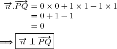
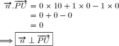
2. a. Montrons que le vecteur est orthogonal
à deux vecteurs non colinéaires et du plan (PQU).
Manifestement, les vecteurs et ne sont pas colinéaires.
De plus,
Par conséquent, le vecteur étant orthogonal
à deux vecteurs non colinéaires et du plan (PQU),
nous en déduisons que le vecteur est normal au plan (PQU).
2. b. Nous savons que tout plan de vecteur normal admet une équation cartésienne de la forme ax + by + cz + d = 0.
Puisque le vecteur est normal au plan (PQU), nous déduisons qu'une équation cartésienne du plan (PQU) est de la forme y - z + d = 0.
Or le point P(0 ; 10 ; 0) appartient au plan (PQU). Ses coordonnées vérifient l'équation du plan.
D'où 10 - 0 + d = 0 , soit d = -10
Par conséquent, une équation cartésienne du plan (PQU) est
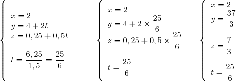
3. Les coordonnées du point I sont les solutions du système composé par les équations de la droite (AB) et du plan (PQU),
soit du système :
D'où les coordonnées du point I sont
4. Les ordonnées de tous les points appartenant à l'obstacle PTQU sont comprises entre 10 et 11.
Or l'ordonnée du point I est égale à est supérieure à 11.
Par conséquent, en suivant la trajectoire (AB), le drone d'Alex ne rencontrera pas l'obstacle.
Partie B : Distance minimale entre les deux trajectoires
1. En utilisant la relation de Chasles, nous obtenons :
Calculons les coordonnées des vecteurs , et
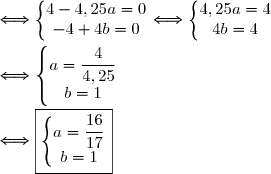
2. La droite (MN) est perpendiculaire à la fois à la droite (AB) et à la droite (CD) lorsque le vecteur est orthogonal aux vecteurs et
Par conséquent, la distance MN est minimale lorsque et
3. Nous avons montré dans la question 1. que les coordonnées du vecteur sont .
Remplaçons a par et b par 1.
Nous savons par l'énoncé qu'une unité correspond à 10 m.
Par conséquent, la distance minimale MN est environ égale à 0,485 10 mètres, soit 4,85 mètres.
Puisque cette distance minimale est supérieure à 4 mètres, la consigne est respectée.
4 points
exercice 3 : Commun à tous les candidats
Par conséquent, l'affirmation 1 est fausse.
Par conséquent, l'affirmation 2 est vraie.
Alors
D'où les vecteurs et sont colinéaires. Les points O, S et T sont donc alignés.
Par conséquent, l'affirmation 3 est vraie.
représente la somme S des n premiers termes d'une suite géométrique de raison et de premier terme .
Par conséquent, l'affirmation 4 est vraie.
5 points
exercice 4 : Candidats n'ayant pas suivi l'enseignement de spécialité
Partie A
1. Arbre pondéré illustrant la situation :
2. Nous devons déterminer
3. a. En utilisant la formule des probabilités totales, nous obtenons :
3. b. 16,2% des téléspectateurs ont regardé l'émission.
Donc P (E ) = 0,162.
Or nous avons montré dans la question 3. a. que P (E ) = 0,44x + 0,14.
4. Nous devons déterminer
Par conséquent, sachant que le téléspectateur interrogé n'a pas regardé l'émission, la probabilité, arrondie à 10-2, qu'il ait regardé le match est environ égale à 0,5.
Partie B
La variable aléatoire T soit la loi normale d'espérance = 1,5 et d'écart-type = 0,5.
1. Nous devons déterminer P (1 T 2).
A l'aide de la calculatrice, nous obtenons : P (1 T 2) 0,68.
Par conséquent, la probabilité qu'un téléspectateur ait passé entre une heure et deux heures devant sa télévision le soir du match est environ égale à 0,68.
2. Nous devons trouver la valeur de t vérifiant la relation P (Tt ) = 0,066.
Nous savons que P (Tt ) = 0,066 P (T < t ) = 1 - 0,066 = 0,934.
Par la calculatrice, nous obtenons
Nous savons que 2,25 heures = 2 heures + 0,25 heure = 2 heures + 15 minutes.
D'où, 6,6 % des spectateurs ont consacré plus de 2h 15min à regarder la télévision le soir du match.
Partie C
La durée de vie d'un boîtier individuel, exprimée en année, est modélisée par une variable aléatoire notée S qui suit une loi exponentielle de paramètre strictement positif.
L'institut de sondage a constaté qu'un quart des boîtiers a une durée de vie comprise entre un et deux ans.
Nous obtenons alors :
L'usine qui fabrique les boîtiers affirme que leur durée de vie moyenne est supérieure à trois ans, soit que l'espérance E (S ) est supérieure à 3.
Par conséquent, l'affirmation de l'usine est incorrecte.
5 points
exercice 4 : Candidats ayant suivi l'enseignement de spécialité
1. a. Graphe probabiliste complété :
D'après le graphe probabiliste, nous déduisons que
Nous aurions également pu démontrer cette relation en utilisant l'arbre pondéré de probabilité.
En utilisant la formule des probabilités totales, nous obtenons :
Selon l'énoncé, nous admettons que, pour tout entier naturel n , bn +1 = 0,2an + 0,2.
2. a. Pour tout entier naturel n ,
3. Pour tout entier naturel n , on pose Vn = Un - Y.
3. b. Démontrons par récurrence que pour tout entier n strictement positif, Vn = M nV0.
Initialisation : Montrons que la propriété est vraie pour n = 1.
Nous avons montré dans la question 3. a. que pour tout entier naturel n , .
En remplaçant n par 0 dans cette relation, nous obtenons : .
Donc l'initialisation est vraie.
Hérédité : Si pour un entier n fixé strictement positif la relation Vn = M nV0 est vraie au rang n , montrons que cette relation est encore vraie au rang n + 1.
Montrons alors que .
Donc l'hérédité est vraie.
Puisque l'initialisation et l'hérédité sont vraies, nous avons montré par récurrence que pour tout entier n strictement positif, Vn = M nV0.
5. Selon l'énoncé, pour tout entier naturel n , nous admettons que
Nous en déduisons que la probabilité que le temps soit pluvieux au bout de n jours ne peut pas dépasser 0,5.
Publié par malou
le
ceci n'est qu'un extrait
Pour visualiser la totalité des cours vous devez vous inscrire / connecter (GRATUIT) Inscription Gratuitese connecter
Merci à Hiphigenie / malou pour avoir contribué à l'élaboration de cette fiche
Désolé, votre version d'Internet Explorer est plus que périmée ! Merci de le mettre à jour ou de télécharger Firefox ou Google Chrome pour utiliser le site. Votre ordinateur vous remerciera !


=\dfrac{a}{1+\text{e}^{-bx}}\ \ \ \ \ \text{où }x\in[0\, ;+\infty[)
=0,5\Longleftrightarrow\dfrac{a}{1+\text{e}^{0}}=0,5 \\\\\phantom{f(0)=0,5}\Longleftrightarrow\dfrac{a}{1+1}=0,5 \\\\\phantom{f(0)=0,5}\Longleftrightarrow\dfrac{a}{2}=0,5 \\\\\phantom{f(0)=0,5}\Longleftrightarrow\boxed{a=1})
=\dfrac{1}{1+\text{e}^{-bx}}}\ \ \ \ \ \text{où }x\in[0\, ;+\infty[)
=-\dfrac{(1+\text{e}^{-bx})'}{(1+\text{e}^{-bx})^2}=-\dfrac{1'+(\text{e}^{-bx})'}{(1+\text{e}^{-bx})^2} \\\\\phantom{f'(x)}=-\dfrac{0+(-bx)'\text{e}^{-bx}}{(1+\text{e}^{-bx})^2}=-\dfrac{-b\,\text{e}^{-bx}}{(1+\text{e}^{-bx})^2}=\dfrac{b\,\text{e}^{-bx}}{(1+\text{e}^{-bx})^2} \\\\\Longrightarrow\boxed{f'(x)=\dfrac{b\,\text{e}^{-bx}}{(1+\text{e}^{-bx})^2}})
=\dfrac{b\,\text{e}^{0}}{(1+\text{e}^{0})^2}=\dfrac{b\times1}{(1+1)^2}\Longrightarrow\boxed{f'(0)=\dfrac{b}{4}} \\\\\phantom{\text{Or }\ }m_{AB}=\dfrac{y_B-y_A}{x_B-x_A}=\dfrac{1-0,5}{10-0}=\dfrac{0,5}{10}\Longrightarrow\boxed{m_{AB}=0,05} \\\\\\\text{D'où }\ f'0)=m_{AB}\Longleftrightarrow\dfrac{b}{4}=0,05\\\\\phantom{\text{D'où.................. }\ }\Longleftrightarrow \boxed{b=0,2})
=\dfrac{1}{1+\text{e}^{-0,2x}}}.)
 [ par
[ par =\dfrac{1}{1+\text{e}^{-0,2x}}}) .
.=\dfrac{1}{1+\text{e}^{-0,2\times10}}}=\dfrac{1}{1+\text{e}^{-2}}\Longrightarrow\boxed{p(10)\approx0,88})
=\dfrac{1}{1+\text{e}^{-0,2x}}}=f(x))
=\dfrac{0,2\,\text{e}^{-0,2x}}{(1+\text{e}^{-0,2x})^2}})
 , nous déduisons que p' (x ) > 0 pour tout x dans [0 ; +
=-\infty \\\\ \lim\limits_{X \to -\infty} \text{e} ^X=0\ \ \ \ \ \ \ \ \end{matrix}\right.\ \ \ \underset{\text{ par composée (X=-0,2x) }}{\Longrightarrow}\ \ \ \ \ \ {\red{\lim\limits_{x \to +\infty} \text{e} ^{-0,2x}=0}} \\\\\text{D'où, }\lim\limits_{x \to +\infty} \dfrac{1}{1+\text{e}^{-0,2x}}=\dfrac{1}{1+0} =1\\\\\Longrightarrow\boxed{\lim\limits_{x \to +\infty}p(x)=1})
>0,95\Longleftrightarrow\dfrac{1}{1+\text{e}^{-0,2x}}>0,95 \\\\\phantom{p(x)>0,95}\Longleftrightarrow1+\text{e}^{-0,2x}<\dfrac{1}{0,95} \\\\\phantom{p(x)>0,95}\Longleftrightarrow\text{e}^{-0,2x}<\dfrac{1}{0,95}-1 \\\\\phantom{p(x)>0,95}\Longleftrightarrow\text{e}^{-0,2x}<\dfrac{1-0,95}{0,95} \\\\\phantom{p(x)>0,95}\Longleftrightarrow\text{e}^{-0,2x}<\dfrac{0,05}{0,95} \\\\\phantom{p(x)>0,95}\Longleftrightarrow\text{e}^{-0,2x}<\dfrac{1}{19} \\\\\phantom{p(x)>0,95}\Longleftrightarrow\ln(\text{e}^{-0,2x})<\ln(\dfrac{1}{19}) \\\\\phantom{p(x)>0,95}\Longleftrightarrow-0,2x<-\ln(19) \\\\\phantom{p(x)>0,95}\Longleftrightarrow x>\dfrac{-\ln(19)}{-0,2} \\\\\phantom{p(x)>0,95}\Longleftrightarrow x>\dfrac{\ln(19)}{0,2} \\\\\text{Or }\ \dfrac{\ln(19)}{0,2}\approx14,7)
=\dfrac{1}{1+\text{e}^{-0,2x}} \\\\\phantom{{\red{4.\ \text{a. }}}\ \text{Pour tout réel }x\ge0, \ p(x)}=\dfrac{1}{1+\dfrac{1}{\text{e}^{0,2x}}} \\\\\phantom{{\red{4.\ \text{a. }}}\ \text{Pour tout réel }x\ge0, \ p(x)}=\dfrac{1}{\dfrac{\text{e}^{0,2x}+1}{\text{e}^{0,2x}}} \\\\\phantom{{\red{4.\ \text{a. }}}\ \text{Pour tout réel }x\ge0, \ p(x)}=1\times\dfrac{\text{e}^{0,2x}}{\text{e}^{0,2x}+1} \\\\\phantom{{\red{4.\ \text{a. }}}\ \text{Pour tout réel }x\ge0, \ p(x)}=\dfrac{\text{e}^{0,2x}}{\text{e}^{0,2x}+1} \\\\\ \ \ \phantom{.............}\Longrightarrow\boxed{p(x)=\dfrac{\text{e}^{0,2x}}{1+\text{e}^{0,2x}}})
=\dfrac{\text{e}^{0,2x}}{1+\text{e}^{0,2x}} \\\\\phantom{{\red{4.\ \text{b. }}}\ p(x)}=\dfrac{{\red{0,2\times}}\,\text{e}^{0,2x}}{{\red{0,2\times}}\,(1+\text{e}^{0,2x})} \\\\\phantom{{\red{4.\ \text{b. }}}\ p(x)}=\dfrac{1}{0,2}\times\dfrac{0,2\,\text{e}^{0,2x}}{1+\text{e}^{0,2x}} \\\\\phantom{{\red{4.\ \text{b. }}}\ p(x)}=\dfrac{1}{0,2}\times\dfrac{(1+\text{e}^{0,2x})'}{1+\text{e}^{0,2x}} \\\\\phantom{{\red{4.\ \text{b. }}}\ p(x)}=\dfrac{1}{0,2}\times\left(\overset{}{\ln(1+\text{e}^{0,2x})}\right)')
=\dfrac{1}{0,2}\times\ln(1+\text{e}^{0,2x}).)
![{\red{4.\ \text{c. }}}\ m=\dfrac{1}{2}\int\limits_{8}^{10}p(x)\,dx=\dfrac{1}{2}\left[\overset{}{P(x)}\right]\limits_{8}^{10}=\dfrac{1}{2}\left[\overset{}{\dfrac{1}{0,2}\times\ln(1+\text{e}^{0,2x})}\right]\limits_{8}^{10} \\\\\phantom{{\red{4.\ \text{c. }}}\ m}=\dfrac{1}{0,4}\left[\overset{}{\ln(1+\text{e}^{0,2x})}\right]\limits_{8}^{10} \\\\\phantom{{\red{4.\ \text{c. }}}\ m}=\dfrac{1}{0,4}\left[\overset{}{\ln(1+\text{e}^{0,2\times10})-\ln(1+\text{e}^{0,2\times8})}\right] \\\\\phantom{{\red{4.\ \text{c. }}}\ m}=\dfrac{1}{0,4}\left[\overset{}{\ln(1+\text{e}^{2})-\ln(1+\text{e}^{1,6})}\right] \\\\\phantom{{\red{4.\ \text{c. }}}\ m}=\dfrac{1}{0,4}\ln(\dfrac{1+\text{e}^{2}}{1+\text{e}^{1,6}}) \\\\\Longrightarrow\boxed{m=\dfrac{1}{0,4}\ln(\dfrac{1+\text{e}^{2}}{1+\text{e}^{1,6}})\approx0,86}](https://latex.ilemaths.net/latex-0.tex?{\red{4.\ \text{c. }}}\ m=\dfrac{1}{2}\int\limits_{8}^{10}p(x)\,dx=\dfrac{1}{2}\left[\overset{}{P(x)}\right]\limits_{8}^{10}=\dfrac{1}{2}\left[\overset{}{\dfrac{1}{0,2}\times\ln(1+\text{e}^{0,2x})}\right]\limits_{8}^{10} \\\\\phantom{{\red{4.\ \text{c. }}}\ m}=\dfrac{1}{0,4}\left[\overset{}{\ln(1+\text{e}^{0,2x})}\right]\limits_{8}^{10} \\\\\phantom{{\red{4.\ \text{c. }}}\ m}=\dfrac{1}{0,4}\left[\overset{}{\ln(1+\text{e}^{0,2\times10})-\ln(1+\text{e}^{0,2\times8})}\right] \\\\\phantom{{\red{4.\ \text{c. }}}\ m}=\dfrac{1}{0,4}\left[\overset{}{\ln(1+\text{e}^{2})-\ln(1+\text{e}^{1,6})}\right] \\\\\phantom{{\red{4.\ \text{c. }}}\ m}=\dfrac{1}{0,4}\ln(\dfrac{1+\text{e}^{2}}{1+\text{e}^{1,6}}) \\\\\Longrightarrow\boxed{m=\dfrac{1}{0,4}\ln(\dfrac{1+\text{e}^{2}}{1+\text{e}^{1,6}})\approx0,86})
 .
.\\B(2\,;\,6\,;\,0,75)\end{array}\Longrightarrow\overrightarrow{AB}\begin{pmatrix}2-2\\6-4 \\0,75-0,25\end{pmatrix}\Longrightarrow\boxed{\overrightarrow{AB}\begin{pmatrix}{\red{0}}\\ {\red{2}}\\ {\red{0,5}}\end{pmatrix}})
.)
)
:\left\lbrace\begin{array}l x=2\\y=4+2t\\z=0,25+0,5t \end{array}\ \ \ (t\in\mathbb{R})})
 est orthogonal
à deux vecteurs non colinéaires
est orthogonal
à deux vecteurs non colinéaires  et
et  du plan (PQU).
 )\\Q(0\,;\,11\,;\,1)\end{array}\Longrightarrow\overrightarrow{PQ}\begin{pmatrix}0-0\\11-10\\1-0\end{pmatrix}\Longrightarrow\boxed{\overrightarrow{PQ}\begin{pmatrix}0\\1\\1\end{pmatrix}})
)\\U(10\,;\,10\,;\,0)\end{array}\Longrightarrow\overrightarrow{PU}\begin{pmatrix}10-0\\10-10\\0-0\end{pmatrix}\Longrightarrow\boxed{\overrightarrow{PU}\begin{pmatrix}10\\0\\0\end{pmatrix}})
 étant orthogonal
à deux vecteurs non colinéaires
étant orthogonal
à deux vecteurs non colinéaires  admet une équation cartésienne de la
  est normal au plan (PQU), nous déduisons qu'une équation cartésienne du plan (PQU) est de la forme y - z + d = 0.
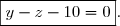
-(0,25+0,5t)-10=0 \end{array}\ \ \ \ \left\lbrace\begin{array}l x=2\\y=4+2t\\z=0,25+0,5t\\1,5t-6,25=0 \end{array} )
}.)
 est supérieure à 11.
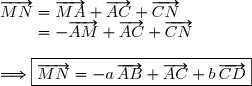
 et
et 
} \\\\\left\lbrace\begin{array}l A(2\ ;\,4\,;\,0,25))\\C(4\,;\,6\,;\,0,25)\end{array}\Longrightarrow\overrightarrow{AC}\begin{pmatrix}4-2\\6-4\\0,25-0,25\end{pmatrix}\Longrightarrow\boxed{\overrightarrow{AC}\begin{pmatrix}2\\2\\0\end{pmatrix}})
\\D(2\ ;\,6\,;\,0,25)\end{array}\Longrightarrow\overrightarrow{CD}\begin{pmatrix}2-4\\6-6\\0,25-0,25\end{pmatrix}\Longrightarrow\boxed{\overrightarrow{CD}\begin{pmatrix}-2\\0\\0\end{pmatrix}})

 est orthogonal aux vecteurs
 +2(2-2a)+0,5(-0,5a)=0 \\-2(2-2b)+0(2-2a)+0(-0,5a)=0\end{matrix}\right. \\\\\phantom{.....................}\Longleftrightarrow\left\lbrace\begin{matrix}2(2-2a)-0,25a=0 \\-2(2-2b)=0\end{matrix}\right.\Longleftrightarrow\left\lbrace\begin{matrix}4-4a-0,25a=0 \\-4+4b=0\end{matrix}\right.)
 et
et 
 .
. et b par 1.
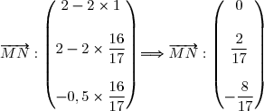
^2+\left(-\dfrac{8}{17}\right)^2} \\\\\phantom{\text{Dès lors}\ MN}=\sqrt{\dfrac{4}{289}+\dfrac{64}{289}}=\sqrt{\dfrac{68}{289}}=\sqrt{\dfrac{4\times17}{17^2}}=\dfrac{2}{17}\sqrt{17} \\\\\Longrightarrow\boxed{MN=\dfrac{2}{17}\sqrt{17}\approx0,485})
 10 mètres, soit 4,85 mètres.
}} \longrightarrow{\red{\text{Affirmation fausse }}})
+\text{i}\sin(\dfrac{\pi}{3})) \\\\\phantom{c=\dfrac{1}{2}\text{e}^{\text{i}\frac{\pi}{3}}}=\dfrac{1}{2}(\dfrac{1}{2}+\text{i}\dfrac{\sqrt{3}}{2}) \\\\\phantom{c=\dfrac{1}{2}\text{e}^{\text{i}\frac{\pi}{3}}}=\dfrac{1}{4}(1+\text{i}\sqrt{3}) \\\\\Longrightarrow\boxed{c=\dfrac{1}{4}(1+\text{i}\sqrt{3})\ {\red{\neq}}\ \dfrac{1}{4}(1-\text{i}\sqrt{3})})

^{3n}=\left(\dfrac{1}{2}\right)^{3n}\,\left(\overset{}{\text{e}^{\text{i}\frac{\pi}{3}\times3}} \right)^{n}=\left(\dfrac{1}{2}\right)^{3n}\,\left(\overset{}{\text{e}^{\text{i}\pi}} \right)^{n} \\\\\Longrightarrow\boxed{c^{3n}=\left(\dfrac{1}{2}\right)^{3n}\,(-1)^{n} \ {\red{\in\R}}}})

^2\Longrightarrow\boxed{z_{\overrightarrow{OS}}=\dfrac{1}{4}\text{e}^{\text{i}\frac{2\pi}{3}}})
}=\dfrac{1}{8}\,\text{e}^{\text{i}\pi}=\dfrac{1}{8}\times(-1)\\\\\phantom{\text{De plus }}\Longrightarrow\dfrac{z_{\overrightarrow{OS}}}{z_{\overrightarrow{OT}}}=-\dfrac{1}{8} \\\\\phantom{\text{De plus }}\Longrightarrow\boxed{z_{\overrightarrow{OS}}=-\dfrac{1}{8}\,z_{\overrightarrow{OT}}})
 et
et  sont colinéaires. Les points O, S et T sont donc alignés.
^n}} \longrightarrow{\red{\text{Affirmation vraie }}})
^2\\...\\|c^n|=|c|^n=\left(\dfrac{1}{2}\right)^n\end{matrix}\right.)
 représente la somme S des n premiers termes d'une suite géométrique de raison
  et de premier terme
 ^n}{1-\dfrac{1}{2}}=\dfrac{1}{2}\times\dfrac{1-\left(\dfrac{1}{2}\right)^n}{\dfrac{1}{2}}=1-\left(\dfrac{1}{2}\right)^n \\\\\Longrightarrow\boxed{|c|+|c^2|+...+|c^n|=1-\left(\dfrac{1}{2}\right)^n})
.)
=P(M)\times P_M(E) \\\phantom{P(M\cap E)}=0,56\times0,25 \\\phantom{P(M\cap E)}=0,14 \\\\\Longrightarrow\boxed{P(M\cap E)=0,14})
= P(M\cap E)+P(\overline{M}\cap E) \\\phantom{P(E)}=0,14+P(\overline{M})\times P_{\overline{M}}(E)\\\phantom{P(E)}=0,14+0,44\times x \\\\\Longrightarrow\boxed{P(E)=0,44x+0,14})
)
=\dfrac{P(M\cap \overline{E})}{P(\overline{E})} \\\\\phantom{P_{\overline{E}}(M)}=\dfrac{P(M)\times P_M(\overline{E})}{1-P(E)} \\\\\phantom{P_{\overline{E}}(M)}=\dfrac{0,56\times0,75}{1-0,162} \\\\\Longrightarrow\boxed{{P_{\overline{E}}(M)}=\dfrac{0,42}{0,838}\approx0,50})
 = 1,5 et d'écart-type
  = 0,5.
 T
T  0,68.
0,68. t ) = 0,066.
 P (T < t ) = 1 - 0,066 = 0,934.
=0,934\Longrightarrow t\approx2,25.})
 strictement positif.
=0,25\Longleftrightarrow P(S\ge1)-P(S\ge2)=0,25 \\\\\phantom{P(1\le S\le2)=0,25}\Longleftrightarrow \text{e}^{-\lambda}-\text{e}^{-2\lambda}=0,25 \\\phantom{P(1\le S\le2)=0,25}\Longleftrightarrow \text{e}^{-2\lambda}-\text{e}^{-\lambda}+0,25=0 \\\phantom{P(1\le S\le2)=0,25}\Longleftrightarrow \left(\text{e}^{-\lambda}\right)^2-\text{e}^{-\lambda}+0,25=0 \\\\\text{Soit }\ X=\text{e}^{-\lambda} \\\text{alors }\ X^2-X+0,25=0\Longleftrightarrow (X-0,5)^2=0 \\\phantom{\text{alors }\ X^2-X+0,25=0}\Longleftrightarrow X-0,5=0 \\\phantom{\text{alors }\ X^2-X+0,25=0}\Longleftrightarrow X=0,5 \\\\X=0,5\Longleftrightarrow\text{e}^{-\lambda}=0,5 \\\phantom{X=0,5}\Longleftrightarrow-\lambda=\ln(0,5) \\\phantom{X=0,5}\Longleftrightarrow\lambda=-\ln(0,5)=-\ln(\dfrac{1}{2}) \\\phantom{X=0,5}\Longleftrightarrow\boxed{\lambda=\ln(2)})
=\dfrac{1}{\lambda}=\dfrac{1}{\ln(2)}\Longrightarrow \boxed{E(S)\approx1,44\ {\red{<3}}})

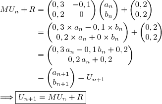
=P(A_n\cap A_{n+1})+P(B_n\cap A_{n+1})+P(C_n\cap A_{n+1}) \\\phantom{P(A_{n+1})}=P(A_n)\times P_{A_n}(A_{n+1})+P(B_n)\times P_{B_n}(A_{n+1})+P(C_n)\times P_{C_n}(A_{n+1}) \\\phantom{P(A_{n+1})}=a_n\times0,5+b_n\times0,1+c_n\times0,2 \\\\\Longrightarrow\boxed{a_{n+1}=0,5\,a_n+0,1\,b_n+0,2\,c_n})
 \\\\\phantom{.............................................................}\Longrightarrow a_{n+1}=0,5a_n+0,1b_n+0,2-0,2a_n-0,2b_n \\\\\phantom{.............................................................}\Longrightarrow\boxed{a_{n+1}=0,3a_n-0,1b_n+0,2})


-({\blue{MY+R}}) \\\phantom{{\red{3.\ \text{a. }}}\ V_{n+1}}=MU_{n}+R-MY-R \\\phantom{{\red{3.\ \text{a. }}}\ V_{n+1}}=MU_{n}-MY \\\phantom{{\red{3.\ \text{a. }}}\ V_{n+1}}=M(U_{n}-Y) \\\phantom{{\red{3.\ \text{a. }}}\ V_{n+1}}=MV_n \\\\\Longrightarrow\boxed{V_{n+1}=MV_n})
 .
. .
. .
.} \\\phantom{\text{En effet }\ V_{n+1}}=M(M^nV_0)\ \ \ \ \ \text{(par hypothèse de récurrence)} \\\phantom{\text{En effet }\ V_{n+1}}=(MM^n)V_0 \\\phantom{\text{En effet }\ V_{n+1}}=M^{n+1}V_0 \\\\\Longrightarrow\boxed{V_{n+1}=M^{n+1}V_0} )
+Y \\\\\text{Or }\ U_0-Y=\begin{pmatrix}a_0\\b_0\end{pmatrix}-\begin{pmatrix}\alpha\\\beta\end{pmatrix}=\begin{pmatrix}1\\0\end{pmatrix}-\begin{pmatrix}0,25\\0,25\end{pmatrix}=\begin{pmatrix}0,75\\-0,25\end{pmatrix} \\\\\text{Donc }\ U_n=M^n(U_0-Y)+Y)
\times0,75+(0,1^n-0,2^n)\times(-0,25)+0,25}} \\\\\phantom{\Longrightarrow a_n}=1,5\times0,2^n-0,75\times0,1^n-0,25\times0,1^n+0,25\times0,2^n+0,25 \\\\\Longrightarrow\boxed{a_n=1,75\times0,2^n-0,1^n+0,25})
=0-0+0,25\\\\\phantom{88888888888888888888}\Longrightarrow\lim\limits_{n\to+\infty}(1,75\times0,2^n-0,1^n+0,25)=0,25\\\\\phantom{88888888888888888888}\Longrightarrow\boxed{\lim\limits_{n\to+\infty}a_n=0,25})

 \\\\\text{Or }0,1^n<0,2^n\Longrightarrow0,1^n-0,2^n<0 \\\\\phantom{\text{Or }0,1^n<0,2^n}\Longrightarrow3,5\times(0,1^n-0,2^n) <0 \\\\\phantom{\text{Or }0,1^n<0,2^n}\Longrightarrow0,5+3,5\times(0,1^n-0,2^n) <0,5 \\\\\text{D'où } \left\lbrace\begin{matrix}c_n<{\blue{0,5+3,5\times(0,1^n-0,2^n)}}\\\\ {\blue{0,5+3,5\times(0,1^n-0,2^n)}} <0,5\end{matrix}\right.\Longrightarrow\boxed{{\red{c_n<0,5}}})
 Voir l'énoncé seul
 forum de terminale